

During the first week of instrumentation, the initial PV system performance was tracked. Figure 28 plots the AC power (watts) sent to the grid by the PV system over several days in April 1998. Sky conditions over the period varied from sunny to partly cloudy to cloudy with rain. Over this short period, the average daily total power to the grid was 15.2 kWh with a peak 15-minute power production of 2.9 kW. When profiled over a daily schedule, the average peak power produced was 2.3 kW at 1:30 EST.
Figure 28.
Module and Array Performance
The maximum peak AC power (2.9 kW) measured is considerably less than the nominal 4.05 kW nameplate rating of the installed system. There are several reasons - all expected. The power production performance of the PV modules is fairly dependent on the array temperature. The higher the panel temperature, the lower the solar to electric conversion efficiency. The Siemens modules installed experience a 0.4% drop in their nominal energy conversion efficiency for each degree centigrade which the arrays are warmer than 25oC. Since array temperature is monitored, a rough correlation with the first week of recorded data shows that module temperatures averaged 55oC at full irradiance (1,000 W/m2) at array tilt. This would indicate the power production performance would be about 88% of the nominal value at full insolation based on temperature influences. A more exact estimate of module performance was obtained through a test that included module and array IV curves.
IV curves from Siemens SP75 module SND5279 were obtained to determine a usable rating versus temperature, Figure 29, and a temperature coefficient. These data indicate that the module rating is about 73 W at 1000 W/m2 and 25oC standard test conditions (STC). Using the derived temperature coefficient from SN D5279, module IV curves from 77 modules were normalized. The average "installed rating" of the 77 tested modules was also about 73 W at STC.
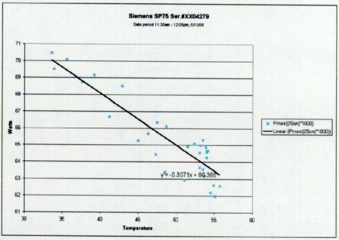
Figure 29. Measured module power output versus temperature.
IV curves were also obtained for the combined arrays. These data were normalized to STC to take into account a number of factors, including mismatch losses, wiring losses, and array surface sloping, all of which will reduce the installed total array rating. When normalized to STC, the data indicate an array rating of 3,523 Watts DC at 1,000 W/m2.
Some 1.3 kW of the 4 nominal kW installed faces the west azimuth. We intentionally installed this segment to explore how this array would assist in meeting late afternoon peak electrical needs for the home. Regardless, its peak power production is somewhat out of phase with that of the larger south facing array (the reason why the observed system peak output is at 1:30 PM rather than noon). This means what when the south system is seeing an insolation level of 1000 W/m2, the west portion will be seeing something less and producing less total peak power. The ratio on the two orientations will change seasonally, but the insolation from the west array averaged 880 W/m2 when the south array was receiving 1000 W/m2. Of course the west array is of advantage in the later afternoon; for example, at 6 PM EST when many homeowners are coming home and turning on appliances, the insolation on array tilt averaged 133 W/m2 on the south array, but was over 250% greater (354 W/m2) on the west array.(9)
Module Operating Temperatures
Within the monitoring protocol, detailed information was obtained on the PV system performance. Measured parameters included the solar irradiance on the horizontal axis as well as on both the array faces (south and west) at their 27 degree tilt. Measured data was also available on ambient air temperatures, roof top wind speed and the center of array module temperatures. On the power production side, data were collected on the direct current (DC) voltage and amperage produced by the array as well as the alternating current (AC) output of the system from the inverter to the utility electric grid.
Since the PV system features a split array configuration, with 2.7 kW facing south and 1.3 kW facing west, the weighted solar irradiance at the respective array tilts can be expected to characterize the majority in the variation in the DC power produced by the array. Figure 30 shows this to be the case. The DC watts produced by the array is approximately 3.15 times the weighted solar irradiance (W/m2) with a coefficient of determination (R-squared) of 0.996. A good portion of the remaining variation was shown to be due to the array module temperatures. For instance a regression based on the weighted array temperatures evidenced a 5.1 W drop in the total system DC power output for every degree oC (9.2 W/oF) which the module temperatures were elevated when exposed to nominal irradiance (800 W/m2).(10) For the system in the Lakeland house, this would indicate a 0.24% drop in PV DC output for each degree increase in module temperature - an approximate estimate that compares reasonably well with the module specifications.
Figure 30. PV system DC output against weighted array irradiance.
Measured module temperatures varied from 7 to 73oC (45
to 164oF) over the April - August monitoring period. They averaged 33oC,
and were closely correlated with the incident irradiance, ambient air
temperature and the roof-top wind speed. The importance of solar irradiance
in elevating module temperatures above ambient is obvious in the relationship
plotted in Figure 31.
The remaining variation due to other factors. At a standard irradiance
of 800 W/m2 (+25 W), the module temperatures averaged 57oC (n=247)
varying strongly with ambient air temperature and wind speed. A regression
of module temperatures against indicated influences showed:
Tmodule = -28.9 + 0.058(Irradiance) + 1.346 (Tambient) -0.351 (Wind Speed)
Where:
Irradiance = W/m2 at array tilt
Tambient = air dry bulb temperature (oF)
Wind speed = roof top air velocity (mph)
R2 = 0.970
Most of the remaining variation was due to the phase lag (thermal capacitance) of the PV array which tended to show warmer than predicted temperatures in afternoon periods immediately following spans with high irradiance and ambient air temperatures and cooler temperatures during morning hours. The data also indicated a strong interaction between the surrounding roof surface temperatures and the PV module temperatures - hardly surprising given the array proximity. With the white tile roof system, the measured maximum south roof surface temperatures at 1000 W/m2 were only 49oC as opposed to 80oC on the asphalt shingles at the Control home. A similar regression to the above that included the measured roof surface temperature showed the roof surface temperature to be a larger influence than the ambient air temperature itself on the predicted module temperatures. This suggests that the white roofing system exerts a beneficial influence on module temperature and overall PV system efficiency.(11)
Figure 31. Elevation in module temperature above ambient air temperature
against array irradiance.
Inverter Performance
On average at 1000 W/m2 of horizontal irradiance, the PV system produced
approximately 2925 W of direct current power. However, the conversion
of DC to AC PV power is of particular importance within the project since
the application is grid connected. The average inverter or Power Conditioning
Unit (PCU) average efficiency from April to August of 1998 was 88%. Since
the project features a split array, the configuration impact on power
conversion efficiency is of interest. One potential problem is the ability
of the inverter to properly power track with the split array. Although
some evidence of this was observed within the data, the overall impact
on power production was minimal.
Figure
32 shows how the inverter AC output over the entire period compares
with the DC input over a range of horizontal solar irradiance. As expected,
the AC output is lower across the span of output, dropping somewhat
by the point that full solar irradiance is achieved (1,100 W/m2) and
as capacity of the inverter is reached. Further illustration of the
system performance is shown in Figure
33. Here, the PCU efficiency is plotted against the DC power output
of the system array. As expected, the conversion efficiency is quite
low at very low DC power levels, the average increasing rapidly to
over 92% by the time 750 Watts of direct current is produced. The performance
then slowly degrades as the maximum conversion capacity (4 kW) is approached.
The question remained, however, as to whether the split array was confounding
the inverter power tracking.
Figure 32. PV system DC versus AC output against horizontal irradiance.
Figure 33. Measured inverter efficiency against PV system DC power
output.
We approached this question in a preliminary fashion by calculating a ratio of the PV power created by the west array to that produced by the south array. This was done by multiplying the relative nameplate ratings of the modules in either direction by the measured array tilt irradiance. To the extent that the west array produced more power than that on the south, the inverter would be faced with different power regimes from the source current of the two arrays. Figure 34 shows how this ratio varied by time-of-day when averaged over the entire monitoring period.
Figure 34. Variation of average inverter efficiency with time-of-day
and relative array irradiance.
As expected, the greatest difference in the power produced by the two arrays occurs during the late afternoon period and to a lesser extent in the morning around 7-9 AM. The graph shows both how the PCU efficiency averaged over time over the entire monitoring period against the ratio of the west/south irradiance. The inverter efficiency rises rapidly during the morning hours, dropping somewhat during mid-day as higher power levels are reached. The unusual dip in inverter efficiency (~5%) seen around 7 PM is likely due to difficulty associated with power tracking when the power produced by the west array varies considerably from that from the south array.
The effect on system power production is minimal, however, since the absolute power produced by the system is low during this period. At 7 PM when the average inverter efficiency drops to 68% the PV system DC output only averages 112 Watts (205 W at 6:45 PM and 43 W at 7:15 PM). This also illustrates an important aspect of the inverter efficiency: the most useful estimate of its efficiency will be based, not on the time-averaged performance of the system, but on the conversion efficiency as weighted by the available DC power. We computed a weighted average inverter efficiency of 89% whereas a time-based average will understate the performance of the power conditioning unit by about 2%. This is because the lowest conversion efficiencies typically occur at low power levels.
Summary Performance
Daily PV power production of the array over the analysis period from April - August averaged 17.64 kWh DC with 15.66 kWh delivered to the utility grid. Over the course of the summer total PVRES building loads (excluding the period subsequent to the installation of the swimming pool pump on August 7th) averaged 22.0 kWh/day so that the PV system produced 71% of the daily electricity required for the building operation. During daytime hours the net impact on the grid is near zero; during evening hours all power required for the PVRES building must come from the utility. Detailed data on the comparative building load profiles and AC power delivered to the grid is produced within the body of the report for June of 1998. The data from this analysis is briefly summarized in Table 6 below:
Table 6
PV System Performance Summary
| Characteristic | May | June* | July | August† | September‡ |
| Horizontal Irradiance (kWh/m2/day) | 6.22 | 6.56 | 5.43 | 5.65 | 3.82 |
| South Irradiance (kWh/m2/day) | 5.90 | 6.03 | 5.12 | 5.61 | 4.00 |
| West Irradiance (kWh/m2/day) | 5.93 | 6.13 | 4.85 | 4.99 | 3.52 |
| Weighted Irradiance (kWh/m2/day) | 5.91 | 6.06 | 5.03 | 5.41 | 3.84 |
| Ambient Air Temperature (oC) | 30.3 | 33.8 | 31.7 | 32.7 | 29.9 |
| Daily Array Efficiency | 9.13 | 9.15 | 9.30 | 7.83 | 9.63 |
| Daily PCU Efficiency | 88.9 | 88.4 | 87.9 | 87.5 | 87.8 |
| Daily System Efficiency | 8.11 | 8.09 | 8.17 | 6.85 | 8.44 |
| House AC Load (kWh/day) | 10.94 | 28.95 | 29.42 | 40.68 | 36.02 |
| AC Energy from Utility (kWh/day) | 3.21 | 12.46 | 15.54 | 28.03 | 25.0 |
| PV AC Energy to Utility (kWh/day) | 8.64 | 0.25 | 0.15 | 0.00 | 0.05 |
| PV AC Energy to House (kWh/day) | 7.73 | 16.49 | 13.88 | 12.85 | 11.02 |
* House occupied on June 4th
† 1 hp (1.8 kW) pool pump installed on August 7th
‡ Pool pump operating all month; averages 12.4 kWh/day with
6.5 hrs of operation
Annual PV System Performance
We used the PVFORM hourly simulation program to predict the annual performance of the PV system and its sensitivity to the off-azimuth orientation of the west-facing sub-array. The PVFORM simulation uses typical meteorological year (TMY) data for solar irradiance and ambient air temperature. Table 7 below shows how the measured and TMY irradiances compare in the three months in the summer of 1998 as well as the measured PV system DC output against that predicted by PVFORM.(12) Two PV forms runs were computed and then combined; one for the south array and one for the west sub-array.
Table 7
Measured and Simulated Performance for PV System
May - July, 1998
| Month of 1998 | Measured Irradiance (kWh) |
TMY Irradiance (kWh) |
Measured DC Output (kWh/month) |
Predicted DC Output (kWh/month) |
| May | 6125 | 6396 | 571 | 607 (581) |
| June | 6270 | 5448 | 568 | 492 (569) |
| July | 5368 | 5590 | 495 | 511 (491) |
The data above indicates that June was sunnier than normal, but data from the other months are similar to typical conditions. Note the relative success of PVFORM in predicting monthly performance even when using TMY data. The predicted values shown in parentheses have been adjusted for the measured differences in the TMY and measured irradiances. Agreement is extremely good, with each prediction within 2% of the measured values.
Based on PVFORM's success in approximating the PV electricity production, we used the model to predict how annual performance would be impacted by the module configuration. The simulation predicted that the split array configuration would produce an annual DC energy power of 6,269 kWh (~5,580 kWh in AC power to the grid). The same simulation predicted the array would have produced 6,604 kWh DC if all 54 modules had been oriented facing south. This indicates that the annual power production penalty from the west facing array was only 4.2%.
Thermal Performance Monitoring
Upon its completion in early April 1998, we noted that with both unconditioned, the PVRES building seemed cooler inside than the Control. Verification of this fact became apparent as soon as instrumentation was installed. Comparative monitoring of the thermal performance of the two homes (Control and PVRES) began on April 15th. Appliances were turned off in both closed-up homes with data recorded for a six day period (April 16th - 20th) in an unoccupied and (mostly) unconditioned state. The data loggers sampled the weather conditions and temperatures around the homes. The two plots below (Figure 35 and 36) show the following measurements taken over the period:
-
Ambient air temperature outside
-
Interior air temperature by the thermostat
-
Temperature of the floor slab at a 2" depth
-
Attic air temperature
Figure 35. Control house thermal performance when unconditioned
Figure 36. PVRES house thermal performance when unconditioned.
Large differences in the attic air temperatures were observed in the two homes - even in mid April. The attic air reaches nearly 120oF in the Control home under its dark brown shingles while the attic under the white tile roof ranges only slightly around ambient air temperature. The interior air temperature in the PVRES home shows much less daily variation than the Control home. The comparison is magnified in Figure 37 which shows that the PVRES home averaged four degrees less than the Control home. The only exception was on Saturday and Sunday when the Control home was air conditioned for several hours by a real estate agent in order to have the interior cool enough to show to prospective buyers (although the PVRES home is sold, the Control home is not). Interestingly, the air conditioning of the Control home was only able to slowly bring its temperature down to the temperature that the PVRES interior was floating at without air conditioning!

Figure 37. Comparative interior temperature conditions in Control
and PVRES homes when unconditioned.
Analysis showed that the long term temperatures in both homes slowly
rose not only, because of the slow increase in daily air temperatures,
but particularly due to the rise in the ground temperature as reflected
in the steady increase in slab temperatures in the first two plots. Infrared
thermography in both homes (Figure 38) showed beneficial heat loss to
the tile/slab floor as opposed to carpeted sections. Measured surface
temperature differences were on the order of 4oF for tiled versus carpeted
sections. Under these spring-time conditions this would indicate a passive
slab heat sink cooling rate on the order of 9,700 Btu/hr had the entire
floor been tiled based on standard surface conductances. This approaches
a ton of "free cooling" available through greater use of tile
rather than carpet and suggests a further improvement to the "minimum
cooling energy building" concept.

Figure 38. Visible and infrared image of section
of flooring where carpet meets tile floor. Note beneficial earth-contact
cooling apparent on tile surface.
In summary, our base monitoring of the thermal performance of the envelopes of the two buildings showed large differences between the two homes - a reflection of the influence of the cooler attic, the exterior insulation on the PVRES home and its high performance windows. So successful did these features appear in concert, that the PVRES building showed little need for air conditioning in late spring. On the other hand, the Control required mechanical cooling to keep its interior temperatures below 80oF when it was shown to prospective customers on week ends.
Unoccupied Cooling Energy Performance
Comparative Cooling Performance in Mild Weather
On April 23rd - 27th the first comparative AC loads were monitored at the PVRES and Control homes under spring conditions. The thermostats were both carefully set to maintain 72oF inside. Since the temperature in April in Central Florida is mild, we set the thermostats artificially low to emulate the temperature differences that will be seen during warmer weather.
The PVRES home maintained an average interior temperature of 71.5oF against 70.8oF inside the Control home. The main reason for the lower temperature in the Control home was that the nighttime temperatures fell lower without the better wall and window insulation levels.
Figure 39 shows the data for the Control home AC power and interior air temperature. Figure 40 shows the same data for the PVRES house. Note that during daytime hours the 4-ton AC at the Control home had difficulty keeping up with the load. The total AC consumption (compressor and air handler) was very different: an average of 19.57 kWh/day in the Control home against 1.79 kWh/day in the PVRES home. The AC consumption in the PVRES home was lower by more than an order of magnitude.
Figure 39. Measured interior temperatures in the Control and PVRES
houses during mild weather conditions.
Figure 40. Measured AC power in the Control and PVRES houses during
mild weather conditions.
Unoccupied Monitoring Under Summer Conditions
Monitoring over the month of May concentrated on direct comparison of
the performance of the unoccupied two homes when air conditioned with
similar thermostat settings. The Control home was set to 76oF in cooling
mode, while the PVRES house was set one degree cooler to insure no favorable
bias. Both homes were left vacant and unattended without appliance loads.
Figure
41 shows the measured cooling load profile on a hot day (May 17,
1998) without the load shift strategy; the Control home has a measured
air conditioning load averaging 3.62 kW during the peak hour between
5 and 6 PM EDST while the PV home has a measured average AC load during
the hour of 0.50 kW - a reduction to the utility coincident peak load
of 86%.
Figure 41. Measured Control and PVRES cooling electric demand
and PV power to grid on May 17, 1998.
At the same time, the average PV power production during the hour average 619 Watts. Total daily electricity consumption for cooling was 37.5 kWh in the Control home against 5.84 kWh in the PV home - a reduction in cooling load of 84%. Moreover, the PV system produced 17.9 kWh which were supplied to the grid with greater power produced than was used during the peak hour. Figure 42 shows a comparison of the net loads of the two new homes when the PV energy is subtracted from the total.
Figure 42. Difference between net demand of Control and PVRES
house on May 17, 1998.
Note that power is sent back to the utility throughout the day with an average difference in load during the peak hours of 4.5 kW. The PV system produced three times as much electricity on this day as the cooling system used (Figure 43).
Figure 43. Comparison of Control and PVRES cooling
energy use against PV system output (May 17, 1998).
The comparative performance over the entire month of unoccupied monitoring showed similar trends. Daily AC use average 42.1 kWh in the control home against 8.7 kWh in the PVRES house - a reduction in space cooling of about 80%.
Evaluation of Load Shift Potential
On June 4th, 1998, the new PVRES owners moved into their new home. After the new owners took occupancy, monitoring continued for the rest of the summer with a load shift strategy utilized. The PVRES home was pre-cooled during the late morning and early afternoon using the Honeywell Chronotherm III thermostat (Figure 44) while allowing the temperature inside to rise during the afternoon hours. Originally, the schedule had been set so that 72oF was maintained from 12 noon through 5 PM with the temperature allowed to rise one degree each hour until 8 PM. However, the occupants found these temperatures too cold and a warmer schedule was agreed upon. On June 11th, we reset the programmable thermostat so that it would pre-cool the building to 74oF between 11 AM and 5 PM and then 76 during the rest of the day in an attempt to shift the load away from the utility peak coincident hours 5 - 7 PM.

Figure 44. Programmable thermostat used for cooling load shift.
Table 8
Load Shift Thermostat Schedule
| Time | Cooling Set Temperature | Cooling Mode |
| 11 AM | 74oF | Pre-cooling period |
| 5 PM | 75oF | Load shift period |
| 6 PM | 76oF | Standard condition |
During the entire period, the thermostat in the Control home remained set at a constant 76oF, although without occupants. The PVRES home had the heat generated by the occupants, appliances and lighting.
In June of 1998, the Central Florida area experienced a record heat
wave and drought which touched off numerous wildfires. The Tampa National
Weather Service - only about 30 miles from Lakeland - reported that the
average June '98 temperature was an all-time record high, for any month
in any year!
Table 9
June 1998 Weather Statistics: National Weather Service, Tampa,
FL
| Average | June 1998 | June 1997 | Relation to Thirty Year Normal |
| Daily Temp. | 85.6oF | 81.8oF | June '98 temp. is 4.3oF above normal 30 year |
| Daily Max. | 93.0oF | 89.7oF | June '98 temp. is 3.5oF above normal 30 year |
| Daily Min. | 78.1oF | 73.8oF | June '98 temp. is 5.2oF above normal 30 year |
Figure 45 shows how the average cooling electric demand in the two homes over the entire month of June. The "load shift" related electric demand increase in the PVRES home (thermostat goes down from 76o to 74o) at 11 AM is very noticeable, as is the drop in load at 5 PM. The total average cooling energy use in the unoccupied Control home is 61 kWh a day ($147 for the month at current utility rates). Even with the internal heat from appliances and occupant the measured cooling was only 18 kWh ($42 for the month) a day in the occupied PVRES house - a reduction of 70%. When total power from the occupied PVRES home is considered (30.3 kWh/day), it still uses only 50% of the air conditioning of the Control.
Figure 45. June cooling energy use profiles in control and PVRES houses.
Figure 46 shows the average daily AC electric consumption (61 kWh/day) at the Control house compares with the PV electric power production (15.6 kWh/day) at the PVRES home. The green line shows the PVRES Net power demand (Total electric load - PV power to the grid). Note that the late afternoon PV electric production was sufficient to approximately zero out the total PVRES electric demand during the peak hours between 4 and 6 PM EST (5 and 7 PM EDT). The total daily net power total use of the PVRES home is only 24% of that of air conditioning alone at the Control.
Figure 46. June net loads and PV power production at Control
and PVRES homes.
Comparison to Neighboring Conventional Homes
Within the PV portion of the project, two additional homes were monitored in the same immediate neighborhood as the PVRES and Control houses. Both were constructed by the same builder and are very similar in size, features and construction to the Control home. PV House #1 has a 2 kW utility integrated south facing PV array and PV House #2 has a similar 1.8 kW PV array. Both were monitored to provide data on PV power and total household electric demand. Figure 47 shows PV#1 and its position relative to the Control home; the PV array installation on house #2 is shown in Figure 48.
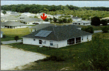
Figure 47. PV house #1, nearby control home directly behind it.
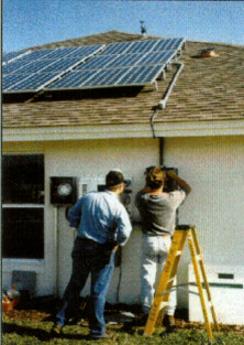
Figure 48. Lakeland Electric and Water assists with field wiring
of PV house #2.
Neither home has any special energy savings measures, but are within one block of the Control and PVRES house. The fact that both homes were occupied provides an interesting comparison with the PVRES home and unoccupied Control home. Table 10 shows a comparison of total electricity consumption, monthly cost and PV Array output in the month of June, 1998.
Table 10
Comparison of All Homes for June 1998
| Site Description | Power Use (kWh) | Monthly Cost
($) |
PV Array Output AC kWh |
Percent PV Output
of Total Loads |
| PVRES | 837 | $ 67 | 502 | 60.0% |
| Control | 1,839* | $147 | None | 0.0% |
| PV#1 | 2,970 | $260 | 255 | 8.6% |
| PV#2 | 2,435 | $195 | 224 | 9.2% |
* air conditioning only
Figures 49, 50 and 51 show a comparison of the total loads and PV output for each of the three homes with PV over the month of June. Both the table and graphs clearly show the importance of efficiency in making the PV output of the systems meaningful relative to total power demand. Whereas the solar electric system in the PVRES home provides 60% of total electrical needs, the smaller system in the other two homes provide only about 9% of total electricity consumption.
Figure 49. PVRES total loads (green) and PV output (red) for
June 1998.
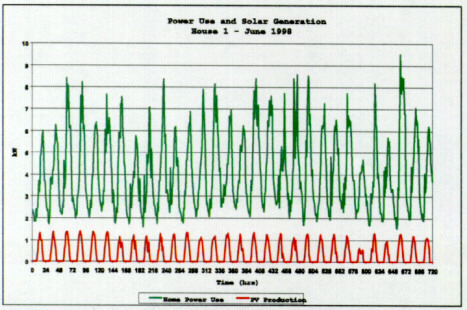
Figure 50. PV house #1 total loads (green) and PV output (red)
for June 1998.
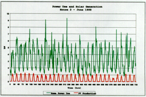
Figure 51. PV house #2 total loads (green) and PV output (red)
for June 1998.
A recent report issued by the Electric Power Research Institute (EPRI) further underscores the importance of building efficiency, load shift and array orientation in the making PV contributions meaningful to controlling utility peak cooling loads. Within this research, 2.3 - 3.2 kW PV arrays were used to power 3 - 5 ton variable speed heat pumps at four monitored test sites in Arizona, Texas and North Carolina. The initial findings showed that the PV arrays were only able reduce space cooling demand by only 15% under peak conditions [21].
On June 18, 1998, Lakeland Electric and Water experienced their maximum annual utility summer peak for the summer, recording a record one-minute demand of 578 MW at 5:03 PM. Figure 52 shows the correspondence between the ambient air temperature measured at the Lakeland test site and the recorded average 15-minute electric demand for Lakeland Electric and Water.
Figure 52. Association of ambient air temperature and utility
system demand on peak summer day.
Maximum recorded ambient air temperature was 100oF (a record) with bright sunny conditions.(13) Figure 53 shows that the Control home used 71 kWh on this day - with the 4-ton air conditioner running constantly between 11 AM and 6 PM. Meanwhile, the 2-ton AC in the PVRES home only runs constantly for the one hour from 11 AM to noon while it pre-cools the building from 76o to 74o and only uses 20 kWh - a 70% reduction in cooling. During the utility peak two hour period it ran less than half the time (908 W) with a demand difference between the homes of 3.82 kW.
Figure 53. Measured cooling energy use in Control and PVRES house
on utility peak day.
Interior comfort conditions show (Figure 54) that the PVRES home was also better able to maintain space conditions. Running constantly from 11 AM onward, the Control home AC was unable to maintain interior temperature conditions at its 76o set point. The recorded interior temperature slowly rose to a maximum of 79.9oF. Meanwhile, the PVRES home easily maintained 74oF during this period. Both the Control and PVRES homes were able to maintain interior relative humidity below 50% during the daytime period even though the PVRES home was occupied and the Control was not.
Figure 54. Measured interior comfort conditions in Control and
PVRES homes on peak day.
The PVRES home was occupied on the peak day while the Control home is not. Even though not comparable, Figure 55 shows that the daily total electricity consumption (33 kWh) in the PVRES home was less than half the air conditioning load alone at the Control. Non-cooling loads at the PVRES home, consisting mainly of refrigeration, lighting and plug loads, totaled 13 kWh about 40% of total consumption.
Figure 55. Measured total loads on Control and PVRES homes on
utility peak day.
Figure 56 on the top of the next page shows how solar photovoltaic (PV) power production affects peak day performance. PV electrical generation sent to the grid totaled 15.6 kWh. Net energy demand of the home (Total Load - PV power) shows that most utility electricity use (15.2 kWh) occurred during the evening hours. PVRES net demand during the two hour utility peak coincident period varied around zero with power used during some periods and sent back to the grid during others. Average peak period PVRES net demand was 225 Watts with a measured average difference against AC use in the Control of 4.5 kW - a peak demand reduction of 95%.
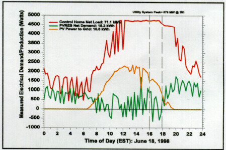
Figure 56. Net utility loads and PV power production in Control
and PVRES homes on utility peak day.
_____________________
9. This west facing portion
of the array may help us to meet our objective of reducing the home's
utility coincident peak demand which typically comes between 4 and
6 PM on summer days.
10. This characterization
was made at the nominal irradiance (800+25 W/m2) over the monitoring
period (n=247 observations). It should be pointed out that the coincident
weather conditions at this irradiance over the monitoring period in
Lakeland, Florida average 31.2oF with a wind speed of 2.1 m/s. The
nominal operating conditions (NOC) are an irradiance of 800 W/m2 with
an ambient temperature of 20oC and a wind speed of 1 m/s.
11. The regression of
module temperature with roof surface temperature added to the prediction
showed considerable improvement in predicting the variation in module
temperatures:
Tmodule= 5.39 + 0.0186(Irradiance) + 1.183(Troof) - 0.250 (Tambient)
- 0.403 (Wind speed)
R2 = 0.993
This relationship would indicate that a white roof surface which runs
33oC cooler under peak conditions than a dark shingle roof would result
in module operating temperatures which were approximately 6oC cooler.
At the manufacturer's specification, this would increase module operating
efficiency by about 2 %.
12. The normalized array
rating for the simulation was based on measured IV curves which indicated
a total array rating of 3,523 Watts at standard test conditions (STC).
13. The City of Lakeland
reported that 101oF was reached.
© 2007-2014 University of Central Florida. The Florida Solar Energy Center (FSEC)
is a research institute of the
University of Central Florida.
For more information about FSEC, please contact us or learn more about us.
Find us on Facebook!