

Measured Conductive Heat Gain to Thermal Distribution System
Within both the Control and PVRES buildings, thermocouples recorded
the temperature of the cooling air leaving the air conditioner evaporator
as well as the temperature of the air when it reached the exit at the
furthest register from the air handler. Approximately half of the mean
difference between could then be used to gauge the average heat gain
to air within the duct system.(2) This
measurement was important since it allowed assessment of the advantage
of the interior mounted duct system in the PVRES home. We predicted that
the heat gain to the duct system would show association with the measured
attic air temperature in the control home. The duct system in the Control
home consists of R-6 flex duct located in the attic space. Based on detailed
work done at FSEC and elsewhere, the surface area of conventional duct
systems are often about a third of the gross floor area of the building
[11].(3)
Figure
13 shows that heat gain to the duct system of the Control home
rose linearly with the measured attic air temperature. A regression
line through the trend showed that the temperature rise from the evaporator
to the far duct register would increase 0.084 degree (oF) for each
degree which the attic air temperature rose. Since maximum attic air
temperature of 140oF was measured, this would indicate a corresponding
duct temperature rise of 7.3oF. Assuming the typical register exhibits
half this heat gain (less distant from the evaporator), the maximum
system heat gain would be 3.65oF. Since the air handler flow was measured
at 1,555 cfm, the computed sensible heat gain under peak conditions
would amount to 6,130 Btu/hr or about half a ton of lost cooling. The
measured sensible energy efficiency ratio of the Control house cooling
system was approximately 6.4 Btu/W. This would indicate an added
electrical load on the cooling system of 960 W under peak conditions.
The negative intercept (-4.46) also has physical significance since
it indicates that the duct system would cease gaining heat from the
attic when the attic air temperature reaches 53.1oF - an indication
of the evaporator leaving air temperature.
Figure 13. Measured register temperature rise versus attic air
temperature in the Control home over the entire summer.
Figure 14 shows how the heat rise of the duct system air in the control home mirrors the attic air temperature conditions on the peak utility day of June 18th, 1998. The average temperature elevation on this particular day is 4.7oF with a daily machine run-time of 64%. This would indicate that losses from the duct system to the attic are responsible to a total increase in the sensible cooling load of 60,500 Btu over the day or an increase in cooling energy use of 9.5 kWh at the measured sensible equipment EER. Since measured total cooling energy was 71 kWh, heat gains to the duct system were responsible for about 13% of total peak day AC load.
Figure 14. Measured duct heat gain against attic air temperature
on the utility peak day.
Carrying out a similar analysis for the entire month of June showed
conductive heat gains to the duct system responsible for about 10% of
the 61 kWh per day of space cooling required.(4) Measured
heat gain to the duct system in the PVRES home from the evaporator to
the far register was about half of that measured in the Control home.
However, since the gains removed heat from the conditioned space of the
home, they did not exert the 10 - 13% penalty in added space cooling
that the attic duct system produced.
The PVRES home substitutes propane for what are normally electric resistance end-uses in conventional homes. This is done to better allow the PV system to match the home's load. For instance, a simple resistance element in a hot water tank (4.5 kW) demands more electrical input than the entire PV system will be able to provide. Propane was used for the oven/range, the clothes dryer, back-up heating for hot water and a direct-vented fireplace. The Control home contains a standard electric resistance 52 gallon storage tank (Rheem 81V5D) in the garage, rated to use 4,828 kWh/year (actual consumption in Florida should be much lower because of our higher inlet water temperature). However, propane is a fairly expensive fuel (approximately $1.40/gallon or $15/MMBtu in Florida), so we endeavored to reduce propane use by the PVRES home. An important measure was to use a solar water heating system with propane back up. Our objective was to provide 70% solar fraction with the solar water heating system at the PVRES home so that propane use is confined mainly to clothes drying and cooking.
The hybrid solar water heating system was installed in the PVRES home in February by Solar Source, a Clearwater, Florida firm. The system consists of a forty square foot American Energy Technology AE-40 solar collector (shown in Figure 15) mounted on the south side of the home's roof. The collector is rated at an energy production of 45,600 Btu/day at the low temperature (95oF) rating. Parasitic pump power is avoided through the use of a 10W PV panel with an Ivan Labs SID-10 magnetic impeller pump. The collector feeds the solar primary tank, a Lochinvar FTA-082-K with an 80 gallon storage capacity. The storage system is made up of two tanks, a primary solar tank and an A.O. Smith FPSE 40 gallon back-up propane tank (Figure 16). The propane tank is a high efficiency direct vent model with electronic ignition. The back-up propane tank is elevated so that it thermosiphons from the primary solar tank only if the water in the solar tank is warmer than the back-up; otherwise it provides feed water to the back-up tank when hot water is drawn.
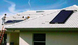
Figure 15. Solar collector for water heating at the
PVRES home.
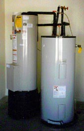
Figure 16. Two tank solar system with propane backup.
We collect data on hot water use (gallons each 15-minutes) as well as electricity use in the control home and propane consumption in the PVRES household. Over the occupied monitoring period, daily hot water use averaged 37.8 gallons per day against a daily propane consumption of only 3.2 ft3 - about 0.09 gallons per day. The installed water heater has a rated energy factor of 0.65 with the measured tap hot water temperature 130oF. Based on measured hot water use and a temperature rise from 80oF to 130oF estimates that propane consumption should be approximately 0.264 gallons/day without the solar assist. This implies a solar water heating fraction of approximately 66%.
Energy-efficient
Lighting
Like most new Florida homes, the PVRES plan features considerable
lighting from recessed cans - thirty in all. In the standard home, each
of these contains a 75W R-lamp incandescent bulb. This connected lighting
load from recessed cans alone of 2.25 kW. Previous research at FSEC has
demonstrated the large savings potential of using compact fluorescent lamps
for residential lighting [9].
In the PVRES home, we took advantage of available compact flourescent lamps (CFL) technology from the Panasonic Corporation. They provided three dozen EFG E15E28 lamps, shown in Figure 17, for installation in the recessed cans of the PVRES home. The lamps fit in the recessed cans which the builder typically uses. It provides virtually identical light output to the 75BR30 lamp and uses only 15 watts (600 Lumens) rather than 75. It also lasts an average of 10,000 hours of use rather than 2,000 for a standard incandescent lamp and thus will seldom need changing. Most importantly, we reduced the connected lighting electric load by almost 80%.
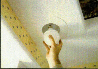
Figure 17. Compact fluorescent globes (15 W) used to
substitute
for incandescent lamps on recessed cans.
After the new occupants had moved into the home on June 4th, several additional CFLs were substituted for existing light fixtures. Table 3 summaries the overall lighting improvements:
Table 3
Lighting System Alterations
| Fixture | Conventional | PVRES | Savings |
| Recessed can lamps (30) | 75 W ea. | 15 W CFL | 1,800 W |
| Table lamp #1 | 100 W | 26 W CFL | 74 W |
| Table lamp #2 | 100 W | 38 W CFL | 62 W |
| Reading lamp | 100 W | 15 W CFL | 85 W |
| Ceiling fan lamp #1 | 60 W | 15 W CFL | 45 W |
| Ceiling fan lamp #2 | 60 W | 15 W CFL | 45 W |
The efficient lighting system lowered the connected lighting load by 2,121 watts - a reduction of 79%. A secondary benefit is the reduced heat produced by the lamps which help to reduce cooling loads. Figure 18 shows a visible and infrared comparison of the two lamp types in the identical fixture in the PVRES and control homes.
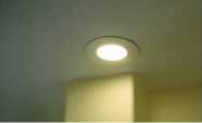

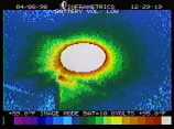
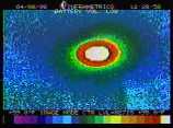
Figure 18. Visible and infrared comparison of light output and
heat produced by the same recessed can in the control and PVRES homes.
In April of 1998, both the PVRES home and the control site were fully instrumented each with a Campbell Scientific CR10 data logger (Figure 19) to both measure weather and thermal conditions, total electrical load, each of the major end-use loads as well as PV system performance. A SW8A pulse count board (top of the enclosure) allows storage of the numerous switch-closure measurements on site. The series of boxes on the swing door are the individual Ohio Semitronics watt-hour transducers that measure the power consumption of the various appliances. Each of the following electrical end-uses were individually metered:
- Total electricity
- Air conditioner
- Air handler
- Hot water
- Refrigerator
- Range
- Dryer
- Washer
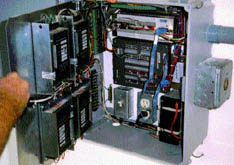
Figure 19. Data logger and power transducers.
Miscellaneous loads, including lighting and ceiling fan use are tracked by subtracting the major electrical end uses from total. Thus, if plug loads were altered, the differences in the estimated miscellaneous loads could be used to estimate the change based on a pre and post monitoring period.
A weather tower was installed to obtain data on ambient air temperature, relative humidity and solar irradiance. Wind speed is obtained by an RM Young anemometer; solar irradiance is obtained from Li-cor silicon cell pyanometers. Ambient and indoor relative humidities are taken by Vaisala hygrometers. Temperatures were taken in a variety of locations throughout both homes to characterize thermal performance. All temperatures are taken with Type-T thermocouples (0.1oF accuracy):
- Ambient air temperature
- Roof surface temperature
- Decking surface temperature
- Attic air temperature
- Interior air temperature by thermostat
- Return air temperature (just before the coil)
- Supply air temperature (just after the coil)
- Supply air temperature at closest register
- Supply air temperature at far register
- Slab temperature (2" depth)
- Garage temperature
- Cold water line inlet temperature
The temperatures taken before and after the air conditioner coil allow
characterization of cooling system performance; the temperatures taken
at the near and far registers allow assessment of heat gains to the
duct system in the Control home. Other unique information is taken
at the PVRES home to characterize the PV system performance:
- Array plane solar irradiance (south)
- Array plane solar irradiance (west)
- Array center temperature (south and west)
- PV DC output voltage
- PV DC output amps
- AC inverter output Watts
Also, the PVRES home has propane used for its range, dryer, a fireplace and back-up for the water heating system. The consumption of the individual propane appliances is recorded by signals sent from the data logger by pulse-initiating AC-250 propane meters provided to the project by the American Meter Company.
All of the data channels in both houses are scanned every ten seconds with integrated averages output to storage each 15-minutes. The resulting data is then sent to FSEC over dedicated telephone lines each evening.
An important objective in selecting the cooling equipment for the PVRES
home, was to take advantage of the features designed to reduce cooling
loads. We used RHVAC (Elite Software) to calculate
the cooling system size for both the standard home and the control home. RHVAC uses Manual
J for its calculations. We entered the building features for either
house in detail (walls, roof, glass, duct system etc.), but as a conservatism
we chose an 95oF outdoor design temperature rather than the 91oF, suggested
by Manual J, along with a 75oF interior temperature. The Manual
J calculations indicated a cooling system of 3.88 tons for the standard
home (4 tons) and 1.73 ton (2 tons) for the PVRES house.
Although, the two ton system for such a large home (2,425 square feet)
is highly unusual, Ward's Air Conditioning in Lakeland and the
Orlando and Tampa Trane offices worked with FSEC to come up with a suitable
system. In a related project, we had a very good experience with Trane's
XL 1400 series air conditioner [16]. Consequently, we selected the TWY024A two-ton
heat pump for the project. We used the TWE040E13 variable speed
indoor air handler to provide optimum efficiency, humidity removal and
quiet operation. The Seasonal Energy Efficiency Ratio (SEER) of the combination
is 14.4 Btu/W; the analogous Heating Season Performance Factor (HSPF)
is 8.5 Btu/W. For the standard home we utilized the a standard efficiency
4-ton Trane heat pump which the project builder typically installs
in his homes - a TWR048C (SEER = 10.0 Btu/W; HSPF = 7.0 Btu/W).
The two units are shown in Figure
20; note the larger size of the condenser for the smaller, more efficient
unit at the PVRES house.
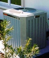
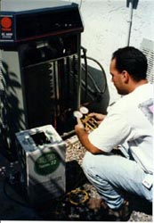
Figure 20. Outside condenser unit used in the Control home
(left)
and PVRES home (right).
Air Conditioner Performance Testing
After each air conditioner was installed, we performed tests on April 8, 1998 to establish the relative performance of each. We developed a procedure entirely based on physical measurements, that can be used to measure the instantaneous efficiency of a cooling system. First the dry coil air flow is determined by turning on the heat pump back-up resistance heat elements and measuring the temperature rise across the heating coil. We used a portable Cooper Instrument Corp. SH66A multi-probe digital thermometer to do take this measurement (Figure 21). By simultaneously measuring the element wattage (we turned off all non-AC breakers and measured this using the utility meter), the air flow cfm can be gauged through knowledge of air's specific heat and density. As a check, we used a Shortridge flow hood to verify the estimate obtained by the resistance heat method (Figure 22).(5)
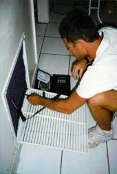
Figure 21. Use of portable temperature measuring equipment to
estimate coil air flow.
Figure 22. Coil air flow is measured with a flow hood.
Secondly, the air conditioner is set on to cooling and the temperature drop measured across the coil. Within the tests, we used two temperature probes before and after the coil. One set of the probes recorded the dry bulb temperature. The other two probes had water saturated cotton shoe-laces inserted into the air stream to measure the wet bulb temperatures before and after the coil. This would allow determination of the AC latent performance by looking at the change in enthalpy across the evaporator coil. As a check on this measurement, we also collected air conditioner condensate over a ten minute period once flow had begun. Finally, an outdoor temperature is taken at the condenser inlet since the rated EER of units is typically based on this condition and that indoors. The product of the change in enthalpy across the evaporator coil times the measured air flow yields the total cooling. By measuring the power demand of the AC system, the system energy efficiency ratio (EER) is obtained.
The measured air flow for the four ton heat pump at the Control house was 1,555 cfm or about 390 cfm/ton. This is well within the tolerance established for the air conditioner (400 cfm/ton). A 16.5 degree temperature drop was measured across the coil (Treturn = 69.2o; Tsupply = 52.7o; Treturn, wet = 59.4o; Tsupply, wet = 50.8o). The measured sensible cooling capacity of the unit at a 77.4o degree outdoor temperature was 26,680 Btu/hr; the latent cooling capacity was 8,560 Btu/hr for a total capacity of about 35,240 Btu/hr. With a 4,181 Watt power draw; this works out to an EER of 8.4 Btu/W. This is short the nominal SEER of 10 Btu/W, but the indoor temperature was much lower (69.2oF) than the 80o assumed in the ARI test procedure.
The test at the PVRES home was done with the variable speed air handler (VSAH) operating at full speed. The unit was configured with the VSAH operating much of the time it operates at less than half speed since measured on cycles last about six minutes.(6)
Within the test, we wanted to evaluate the unit operating at maximum speed where sensible heat gain would be at its highest and latent heat removal at its worst (a chronic problem in Central Florida). At full speed we measured an air flow of 1,380 cfm (690 cfm/ton). The unit was operated in this mode for 20 minutes before measurements were taken; the outdoor inlet air temperature was 87oF. A 12.9 degree temperature drop was measured across the coil (Treturn = 70o [62oW.B], Tsupply = 57.1o [56oW.B.]) with a sensible cooling rate of 18,530 Btu/hr. Even at the high flow rate, latent performance was quite good with 8,770 Btu/hr of moisture removed. Total capacity was 27,300 Btu/hr with measured power at 2,074 Watts - an overall EER of 13.2 Btu/W. The nominal SEER of the specific unit is 14.5 Btu/W. The rated capacity of the unit at the closest rated condition (85oF outdoor dry bulb, 72oF entering dry bulb, 63oF wet bulb) was 25,200 Btu at 900 cfm with an EER of 14.1 Btu/W. Given the higher outdoor temperature, the unit was close to its rated efficiency.
Air infiltration can represent a major cooling load in Florida's hot and humid climate. We used a Minneapolis blower door (Figure 23) to measure house tightness in both homes on April 22, 1998. For the Control home the total overall building tightness of the control house was 2,025 CFM50 or 6.3 ACH50 with a house equivalent leak area (ELA) of 95.2 square inches. The overall tightness of the PVRES home was 1587 CFM50 or 4.9 ACH50 with a house ELA of 69.0 square inches. For Central Florida's climate, a useful rule of thumb to determine the house natural air infiltration rate is to divide the house ACH at 50 pascals by 30. This would estimate a typical natural air change rate of about 0.16 ACH in the PVRES home and 0.21 ACH in the Control. In both homes, we noted that much of the leakage to the outside appears to be from the 30 recessed lighting cans in the ceiling.
Figure 23. Blower door test used to determine house tightness
We used a Duct Blaster™ (Figure 24) testing device to determine the relative leakage in the return and supply sides of the duct systems in both homes. In the Control home, the total CFM25 leakage of the duct system to outside the conditioned space was 122 CFM25. Given its 2,425 square feet of conditioned area, the duct leakage to outside is 0.05 cfm/ft2. This compares to the 0.03 cfm/ft2 proposed as a standard for utility new homes programs. In the PVRES home, the total CFM25 leakage of the duct system from outside the conditioned space was 50 CFM25 or about 0.021 cfm/ft2 - a low value.
Figure 24. Duct leakage is tested in the PVRES house.
In summary, we found that the tightness of the duct system of the Control
home was very average relative to most homes which we have tested. One
limitation of the test, however, is that with the air handler operating,
all the leaks are not the same. Ceiling penetrations close by the air
handler can bring air from the attic -- air that is super heated in the
Control home. Moreover, any of the 50 cfm air that is unintentionally
drawn from the attic is being taken from a space that typically gets
no hotter than the outside ambient air temperature. The PVRES home, with
its interior duct system, on the other hand, had as low a leakage to
the outside of the building of any that have been tested by FSEC.
Evidence of unintended air leakage in the Control home from the attic
to the air handler casework in its interior closet was clearly seen in
infrared thermography on the air handler (Figure 25). This is contrasted
by the lack of such leakage with the interior duct system in the air
handler case itself suggests that ceiling penetrations by the air handler
closest will lead to air being drawn from the space. It also suggests
the great hazard of allowing air handlers to be located within attic
spaces.
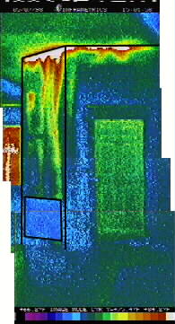
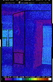
Figure 25. Comparative thermographs of air being drawn
from the attic to the air handler in the Control house (center). The
interior duct system in the PVRES house shows no problem of this type.
Our test results indicate a fairly tight building envelope for both
homes, with the PVRES home somewhat better. However, the leakage duct
systems for the two homes show large differences, mainly due to interior
duct system in the PVRES site. Moreover, thermography showed that the
leakage from the attic to the air handler at the Control site has disproportionate
impact on cooling efficiency.
Measured Building Air Infiltration Rates
To supplement the blower door test, we evaluated the in situ air
infiltration rate in both homes using sulfur hexafluoride (SF6) tracer
gas decay. The blower door indicated that the PVRES home was tighter
with less leakage area, but how the tightness will impact actual air
leakage rates is strongly influeanced by the operating pressures within
the building, particularly when the mechanical air distribution system
is operating.
Both homes were evaluated on May 20, 1998 with the air handler on and
off. The tracer gas concentration decay was measured by two Bruel & Kjaer
Model 1302 multi-gas monitors over a one hour period subsequent
to SF6 injection. The air handler off test provides information
on the "natural air infiltration rate" from air leakage driven
by temperature differences and wind on the external building envelope.
The air handler on test shows how operation of the mechanical
air handler equipment can impact the overall building leakage rate in
air changes per hour(7).
Past studies have shown that operation of the air handler will typically
increase building air leakage rates by two to three time the "natural" rate
which is typically low in Florida homes due to the small driving forces
(bouyancy and wind) [10]. However, we would expect the interior duct
system in the PVRES home to somewhat reduce the relative impact.
Table 4
Measured House Air Infiltration Rates
SF6 Tracer Gas Decay Test
Case |
AH |
Air Changes |
Interior Temp |
Exterior Temp |
Wind Speed |
| Control | Off |
0.131 |
76 |
90.6 |
5.2 |
| Control | On |
0.349 |
76 |
89.9 |
8.0 |
| PVRES | Off |
0.085 |
74 |
86.5 |
9.5 |
| PVRES | On |
0.131 |
74 |
85.6 |
10.2 |
The PVRES home evidenced tighter construction in all cases the air change
rates were low. The natural infiltration rates (air handler off) were
0.085 and 0.131 ACH in the PVRES and Control homes respectively. The
air change rates with the air handler operating was 0.131 in the PVRES
and 0.349 in the Control revealing that the air handler operation increased
building air leakage by 54% and 266% respectively.
It is important to note that in all the cases the building ventilation
rate was low relative to the recommended rates within ASHRAE standard
62-1989 of 0.35 ACH [17]. However, it cannot be argued that the
higher infiltration rates for the Control home are better, since much
of the infiltration air is coming from an undesirable location (the hot
attic). The data do suggest, however, that some system of mechanical
ventialtion with heat and enthalpy recovery may be desirable for future
homes of this type.
Utility
Interactive Photovoltaic System
The photovoltaic (PV) solar electric generation system is grid-interactive, producing DC power which is inverted into AC current and then directly fed into the local utility feeder of Lakeland Electric and Water Company. FSEC researchers developed the specifications for a utility interactive photovoltaic (PV) system to be used for the study. Hutton Communications, Inc. was selected as the systems integrator and was tasked with providing a ready-to-install kit. Hutton selected the system components including the photovoltaic modules and power conditioner. They provided assurance of compatibility between the various products and supplied most of the minor components, which included schematics for the electrical connections, junction boxes, fuse blocks, and lightning suppressors.
Sizing the Photovoltaic Array
The PV generation system was sized to provide power that would offset
as much of the household loads as possible. The PV Forum simulation
model [18] provided an estimate of the usage and the PV array output. Based
on the predicted loads for a peak day, a 4 kW solar array was specified.
An array this size requirements of a 4 kW array. Also, previous simulation
analysis in Japan had shown that a more westernly array facing would be
beneficial in that climate to meet cooling and heating needs [19]. Based
on our own analysis this also looked to be the case in Florida. It was
determined that the array would be split into 2 sub-arrays, one facing
south and the other facing west. This setup allows the total number of
modules installed to remain the same but significantly changes the generation
profile of the array. Simulation models indicated that the west-facing
array would be slightly less efficient at utilizing the solar radiation
for this application because of the orientation; but the west sub-array
would generate appreciable power later in the day, after the output of
the south sub-array had diminished and when power generation is most important
to the utility. The roof top array configuration is illustrated in Figure
26.
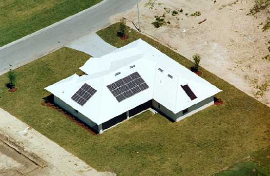
Figure 26. Roof-top split PV array configuration on the PVRES
home.
A Utility Interactive System
The photovoltaic system in this study is owned and maintained by the electric utility company; the power generated is supplied to the utility side of the meter. The output this distributed production facility is monitored by the utility company to evaluate the system performance and to troubleshoot problems. Systems installed such as this one increases the capacity of a service provider and can help reduce the total operating hours required for fuel burning generators.
Photovoltaic Modules
Siemens SP75 solar modules were selected for installation on the roof of the house. These single crystalline modules have a maximum power rating of 75W and have a selectable voltage of 12V or 6V. Bypass diodes are installed in each module to minimize the power loss due to partial shading. The photovoltaic arrays were installed in panels, each comprised of three modules connected in series. Thirty-six modules or twelve panels make up the south-facing sub-array (array rating of 2,700 W) and twenty-four modules or six panels face west (rated output = 1350 Wp). The combined total rating of all 55 modules (18 sub-arrays with six source circuits) is 4050 Watts at standard operating conditions.
Inverter/Power Conditioner
A SW4048UPV sine wave AC power inverter from Trace Engineering was selected to convert the DC from the array to AC and interact with the utility grid (Figure 27). This inverter has a 240VAC - 60Hz output and provides high quality power, which is required for utility line-tie applications. Ground-fault interrupt circuitry is provided for protection and the unit shuts down automatically when utility power is lost.
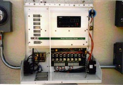
Figure 27. Trace inverter
Monitoring of the comparative performance of the PVRES and Control homes was split during the spring and summer of 1998 into four distinct periods:
- 71oF interior set-point
74oF interior set-point
1) Unoccupied thermal performance: two buildings monitored without space conditioning but with interior temperatures and weather conditions recorded.
2) Unoccupied cooling energy monitoring: two differing cooling energy set points used in periods with similar set points in each home
3) Load shift: A two degree pre-cooling period (11 AM - 5 PM) used in the PVRES home (74o) with a 76o constant thermostat setting in the Control home.
4) Load shift occupied: As above, but with the PVRES home occupied,
but with the Control home unoccupied.
Table 5 shows the average recorded electrical loads for non-space conditioning
at the PVRES home since the home was occupied on June 4th. Appliance
loads are not shown for the Control home since it was unoccupied.
Table 5
Measured PVRES Appliance Energy Consumption
| Appliance | Mean Power | Total Estimated Annual Consumption | |
| Refrigerator | 106.7 W | 935 kWh | |
| Washer | 6.9 W | 60 kWh | |
| Dryer # | 5.7 W | 50 kWh | |
| Range # | 5.8 W | 51 kWh | |
| DHW blower # | 1.7 W | 15 kWh | |
| Lighting, plug loads | 368.8 W | 3232 kWh | |
| Propane End-Uses | Mean Rate | Total Annual | Estimated Annual Propane Gallons |
| DHW burner | 0.134 ft3/hr | 1174 ft3** | 32.3++ |
| Range | 0.030 ft3/hr | 263 ft3 | 7.2 |
| Dryer | 0.053 ft3/hr | 464 ft3 | 12.8 |
** 2,522 Btu/ft3 of propane with 91,500 Btu/gallon; 36.3 ft3/gallon
# Electricity consumption for propane appliances (blowers, ignitors,
motors)
++ Solar primary with propane back-up
All the annual estimates are preliminary and approximate, since they are based on a limited summer monitoring period. Annual hot water consumption and cooking are certain to be larger than the summer measured values, while refrigeration is likely to be lower.(8) The measured daily hot water consumption at the two person household was 37.8 gallons per day. Fireplace propane consumption cannot be estimated since no space heating was required during the monitoring period.
Refrigerator
For the project we attempted to locate one of the Super Efficient Refrigerator Program (SERP) units since we were familiar with their performance from in a previous monitoring project [16]. The 25-cubic foot side-by-side refrigerators feature an advanced compressor, vacuum panel insulation and fuzzy logic defrost control. They also use very little electricity compared with most models with through-the-door features. Sears indicated that although discontinued, they did still have a limited stock of the Kenmore 55792. We soon discovered that the unit could only be sold in the service territory of certain utilities, but Sears tracked down one of the Kenmore units on in San Leandro, California. We then had the unit shipped direct from Sears to Lakeland, Florida. It arrived on October 20, 1997.
Unfortunately, the PVRES house, where the refrigerator was stored, was
broken into on April 28th, 1998 and the SERP refrigerator was stolen.
Again, we went to Sears and obtained the most efficient refrigerator
then available other than the SERP model of the large side-by-side type.
This was the 25 cubic foot Kenmore 57572 model with an estimated
annual energy consumption of 777 kWh/year. The unit was successfully
installed in June of 1998 and its performance has been monitored since.
Over the warmer summer period from June - August, consumption has averaged
2.56 kWh/day - about 20% greater than the nameplate rating. Annual consumption
will likely be lower over the entire year.
________________________
2. The implicit assumption
is that the registers of the duct system are typically located half
of the distance from the evaporator of the furthes duct register.
3. This would indicate
a duct area of about 900 square feet and with R-6 ducts, a heat conductance
of approximately 150 Btu/oF.
4. Duct heat gains are
conservatively estimated in these calculations since gain is estimated
based on machine run-time. In actuality, heat is gained between cycles
as well. Actual annual cooling loads sue to the duct system are likely
9 - 10%.
5. One hint for anyone
performing this test: make sure that the thermometer after the coil
is around the first bend in the duct work, or at the first register,
or you will risk poorly mixed air in the air stream after the coil.
6. For each cooling cycle,
the unit operates at 50% flow for the first minute, then 80% flow for
the next 7.5 minutes and finally 100% flow after that if the thermostat
has not been satisfied.
7. The internal volume
of both the PVRES and Control houses is approximately 22,860 ft3.
8. Typically inlet water
temperatures for water heating vary seasonally by 14oF from approximately
68 - 82oF in Central Florida from a low in January to a high in August.
Also, cooking energy demand is typically greater in the holiday season.
© 2007-2014 University of Central Florida. The Florida Solar Energy Center (FSEC)
is a research institute of the
University of Central Florida.
For more information about FSEC, please contact us or learn more about us.
Find us on Facebook!