

Reference Publication: Parker, D., Huang, Y., Konopacki, S., Gartland, L., Sherwin, J., Gu, L, "Measured and Simulated Performance of Reflective Roofing Systems in Residential Buildings", ASHRAE Transactions, Vol. 104, Pt. 1, American Society of Heating, Refrigerating and Air Conditioning Engineers, 1998. Disclaimer: The views and opinions expressed in this article are solely those of the authors and are not intended to represent the views and opinions of the Florida Solar Energy Center. |
Measured
and Simulated Performance of
Reflective Roofing Systems in Residential Buildings
Danny
S. Parker, Yu Joe Huang, Steven J. Konopacki,
Lisa M. Gartland, Ph.D, John R. Sherwin, Lixing Gu, Ph.D., P.E.
Florida
Solar Energy Center (FSEC) and Lawrence Berkeley
National Laboratory
FSEC-PF-331-98
Abstract
A series of experiments in Florida residences have measured the impact on space cooling of increasing roof solar reflectance. In tests on 11 homes with the roof color changed mid summer, the average cooling energy use was reduced by 19%. Measurements and infrared thermography showed that a significant part of the savings were due to interactions when the duct system is located in the attic space. An improved residential attic and duct simulation model, taking these experimental results into account, has been implemented in the DOE-2.1E building energy simulation program. The model was then used to estimate the impact of reflective roofing in 14 different climate locations around the United States.
Introduction
Traditional architecture in hot climates has long recognized that light building colors can reduce cooling loads (Givoni, 1976). A good example are the recommendations appearing in House Beautiful for climate sensitive residential building practice in South Florida prior to the wide spread adoption of air conditioning (Langewiesche, 1950):
“The White Roof
Your roof must be white. The white color throws much of the heat back into the sky before it ever gets into the roof. This is one climate control idea that is universally accepted in Florida right now...Insulation also is a must, of course, but without the white color, would finally get hot.”
Unfortunately, much of this traditional wisdom has been lost during succeeding air conditioned generations. However, reinforcing the importance of light colors have been a series of simulation and experimental studies demonstrating that building reflectance can significantly impact cooling needs (Givoni and Hoffmann, 1968; Taha et al., 1988; Griggs and Shipp, 1988, Akbari et al., 1990 and Bansal et al., 1992). Full building field experiments in Florida and California over the last five years have examined the impact of reflective roof coatings on air conditioning (AC) energy use in a series of tests on occupied buildings. In Florida, tests were conducted on 11 residential buildings using a before and after test protocol where the roofs were whitened at mid-summer. As shown in Table 1, measured AC electrical savings in the buildings during similar pre and post retrofit weather periods averaged 19% ranging from a low of 2% to a high of 43% (Parker et al., 1995). Even greater fractional savings have been reported for similar experiments in California (Akbari, et al., 1992).
In Florida, cooling energy reductions varied depending on initial ceiling insulation level and roof solar reflectance, the location of the air duct system roof geometry and ventilation and air conditioner size. An example of the large reductions observed in measured attic air temperatures and coincident air conditioner electrical demand is shown in Figure 1.
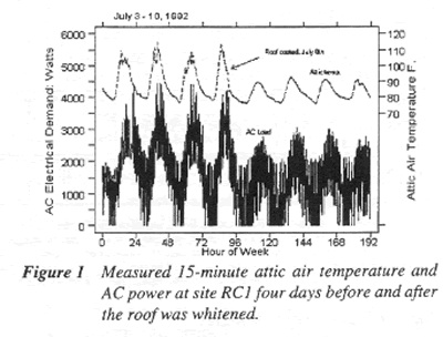
Table 1 Results of Florida Field Tests of Reflective Roofing Systems |
||||||
Test Site |
Reflectance Before |
Reflectance After* |
Cooling Energy
Use (kWh/day) |
Reduction in Utility
Coincident Peak Demand (5-6 p.m.) |
||
Before |
After |
Savings |
||||
| Site 0 Merritt Island, white coating on shingles, concrete block with R-25 ceiling insulation, attic ducts |
0.22 |
0.73 |
38.7 |
34.7 |
4.0 (11 %) |
Not Measured |
| Site 1 Cocoa Beach, white coating on shingles and flat gravel, R-11 attic insulation, attic ducts |
0.21 |
0.73 |
40.6 |
30.3 |
10.3 (25 %) |
661 W (28 %) |
| Site 2 Cocoa Beach, white coating on modified bitumen, flat roof and no attic insulation, attic ducts |
0.10 |
0.73 |
35.5 |
20.1 |
15.4 (43 %) |
858 W (28 %) |
| Site 3 W. Florida, white coating on shingles, no attic insulation, no attic ducts |
0.08 |
0.61 |
22.4 |
16.8 |
5.6 (25 %) |
496 W (30 %) |
| Site 4 Miami, white coating of gravel roof, partial R-11 attic insulation, attic ducts |
0.31 |
0.61 |
51.9 |
43.9 |
8.0 (15 %) |
444 W (16 %) |
| Site 5 Merritt Island, white coating on tile roof, R-7 attic insulation, attic ducts |
0.20 |
0.64 |
57.5 |
45.9 |
11.6 (20 %) |
988 W (23 %) |
| Site 6 Palm Bay, white coating on shingles, R-19 attic insulation, attic ducts |
0.15 |
0.59 |
34.1 |
30.9 |
3.2 (10 %) |
354 W (16 %) |
| Site 7 Palm Bay, white coating on shingles, R-19 attic insulation, attic ducts |
0.22 |
0.64 |
41.1 |
40.2 |
0.9 (2 %) |
304 W (12 %) |
| Site 8 Cape Canaveral, white coating on metal roof, R-11 attic insulation, attic ducts |
N/A |
0.64 |
34.6 |
27.0 |
7.6 (22 %) |
201 W (12 %) |
| Site 9 Cocoa, white coating of gravel roof, R-19 insulation, attic ducts |
0.21 |
0.63 |
32.5 |
28.3 |
4.2 (13 %) |
219 W (11 %) |
| Site 10 Cocoa Beach, white coating of gravel, no insulation, attic ducts |
0.25 |
0.64 |
53.2 |
39.4 |
13.8 (26 %) |
922 W (29 %) |
| Averages | 0.20 |
0.65 |
40.2 |
32.5 |
7.7 (19 %) |
545 W (22 %) |
| * Roof reflectances in the table were measured using an in situ inverted pyranometer method. While a good indicator of relative reflectance, the field method is not so exact as the laboratory test (ASTM-E-903). As example, evaluation of a gray asphalt shingle showed a reflectance using the inverted pyranometer method of 8% which was verified by ASTM-E-903. However, in evaluating the reflectance of twice coated shingles of the same type the laboratory test showed a reflectance of 71% as opposed to 61% for the field measurement. The laboratory measurements should be considered the more valid measurement. For a compilation of laboratory tested surface reflectances see Regan and Acklam (1979); Taha et al., (1992) and Parker et al., (1993B). A discussion of the limitations of the field measurement technique is contained in Lapujade (1994). | ||||||
Simulation Development
The apparent success of reflective roofing in reducing sensible cooling loads in residential buildings has lead to questions regarding the generic applicability of reflective surfaces in different climates. Although effective in Florida and California, how beneficial are white roofs in colder climates where heating energy use may be adversely affected?
To answer such questions, building energy simulations were used. For the study, we chose DOE-2.1E, a widely used building energy simulation program. However, even with this detailed hourly-model, researchers have encountered difficulties in obtaining agreement between measured and simulated savings for white roofs. This problem has been previously explored using DOE-2 for California commercial buildings based on measured and simulated performance (Gartland et al., 1996). However, for residential buildings we desired a model which could simulate a vented attic space and compute the interactions with the thermal distribution system was needed.
A problem with accurately simulating the effect of roof reflectance on cooling energy use has been the inability to adequately simulate interactions between the duct system and the space in which it is located. Duct systems are often located in the attic space in Sun Belt homes. In an early assessment of the impact of reflective roofing, infrared thermography revealed that heat gain to attic-mounted duct systems and air handlers could be adversely affected (Parker et at., 1993). Previous analysis has shown that attic heat gain to the thermal distribution system can increase residential cooling loads by up to 30% during peak summer periods (Parker et al., 1993; Jump et al, 1996). Similarly, Hageman and Modera (1996) found that a large portion of the measured cooling energy savings of radiant barrier systems in field applications can be attributed to reduced heat gains to the thermal distribution system.
To remedy this limitation of the chosen software, a function was written for DOE-2.1E which explicitly accounts for heat transfer to the attic air duct thermal distribution system. Also, a more detailed model of the attic was created which accounts for radiation, ventilation, ceiling framing factors and the changing conductivity of insulation with temperature.
Attic Model
The residential attic was modeled in DOE-2 as a buffer space next to the conditioned residential zone. Experience from previous work on a detailed simulation of attic thermal performance was used to create an appropriate model for DOE-2 (Parker et al., 1991). In the base configuration the roof was modeled as asphalt shingles over felt paper, 3/4" (1.9 cm) plywood decking and engineered trusses. The exterior roof surface assumes a set exterior infrared emissivity (set to 0.90) with the exterior convective heat transfer coefficient computed by DOE-2 based on surface roughness and wind conditions as described by Gartland et al. (1996). Convective and radiative exchange between the roof decking and the attic insulation is accomplished by setting the interior film coefficient according to the values suggested in ASHRAE (1993) dependent on the slope and surface emittance.
The attic floor was assumed to consist of a given thickness of fiberglass insulation over 1/2" (1.3 cm) sheet rock. Heat transfer through the attic floor joists were modeled in parallel to the heat transfer through the insulated section. Framing, recessed lighting cans, electrical junction boxes and other insulation voids are assumed to comprise 15% of the gross attic floor area. The attic is assumed to have soffit and ridge ventilation such that it meets the current recommendation for a 1:300 ventilation area to attic floor area ratio. The rate at which ventilation air enters the attic space is modeled using the Sherman-Grimsrud air infiltration model as previously implemented by Huang (1996). The rates predicted by the model have been compared to previous work in which attic ventilation rates were measured (Parker et al., 1993; Walker et al., 1995). Typical predicted mid-day summer ventilation rates are on the order of 2 - 5 ACH and vary largely with local wind speeds. Site wind speeds for calculating attic ventilation and house air infiltration are estimated assuming typical suburban terrain and shielding factors.
Ceiling insulation conductivity is assumed to be constant within the loads calculations within DOE-2. However, it is widely known that the conductivity of low density insulation is dependent on the mean temperature across the insulation (Turner and Malloy, 1981), and increases with increasing temperature. Since higher roof reflectance can reduce the temperature within the attic space, it was deemed important to model this effect. Based on data from Wilkes (1981) the temperature dependent conductivity of fiberglass insulation rated at 70oF (21.0oC) can be estimated as:
kact = k70°F [1+0.00418 (T-530)]
Where:
k = insulation conductivity (Btu-ft/hr-ft2-°F)
T = is the mean insulation temperature in Rankine.
The influence was implemented within DOE-2 by calculating an hourly correction term based on the interior and attic air temperatures to use to estimate the changing conductivity. The steady state value is then differenced with the hourly estimate to yield a change to the building heating or cooling loads within the systems model. The differences are typically small -- a maximum of a 14% increase in conductance when the attic air temperature reaches 130°F (54.4oC) with 78°F (25.6oC) maintained on the interior. The impact on annual cooling energy use predicted by the model was only 1 to 2% -- similar to that seen in another analysis (Levinson et al., 1996).
Duct Heat Transfer
The authors developed a very detailed simulation of heat transfer to thermal distribution system which was used to guide the development of a simplified function within the systems simulation module in DOE-2.1E which can model this interaction (Parker et al., 1993; Gu, et al., 1996). The following parameters are input:
Supplyarea = Supply Duct Surface Area (ft2)
Returnarea = Return Duct Surface Area (ft2)
SupplyZone = Supply Duct Zone (attic, crawlspace, basement, garage, interior)
ReturnZone = Return Duct Zone (attic, crawlspace, basement, garage, interior)
Rduct = Duct thermal resistance;R-value (4 hr-ft2-°F/Btu)
Heat gain to the duct system is proportional to the duct system thermal conductances, the involved temperature differences and the machine run-time fraction:
UAsupply = Supplyarea / Rduct, supply
UAreturn = Returnarea / Rduct, return
The default areas for the duct system were determined identically as in the ASHRAE SPC 152P work (Gu et al., 1996): the respective surface areas of the duct system are 69 ft2 (6.4 m2) for the return side and 370 ft2 (34.4 m2) for the supply ducts. The supply air temperature and that of each zone containing the ducts is available within the Systems model as well as the average temperature of the return air to that of the interior (78°F or 25.5°C). The heat gain to the duct system is then:
Qduct = (Tzone - Tsupp) * UAsupply + (Tzone-Tint) * UAreturn
Where:
Tzone = Temperatures in which the duct system are located
Tint = Interior air temperature to return system
The fraction of the heat gain to the duct system in an individual hour depends on run time fraction (RTF), which depends on the capacity (Qcap) of the machine (36,000 Btu/hr; 10,552 W) and its EER (10.0 Btu/W or COP = 2.93): 3.6 kW at full run-time fraction. The air conditioner electric demand (ACkW) is directly available as output from the systems section in DOE-2:
RTF = (ACkW / (Qcap/EER*1000))
A first-order correction term must be added to the initial estimate to account for the fact that the machine must run longer to abate the duct heat gains and that the ducts continue to absorb heat in between cycles:
RTF' = RTF + Qduct/ Qcap
The addition to the AC electrical load from the duct system is then:
DuctkW = Qduct * RTF' / (EER*1000)
A similar calculation is made to adjust HVAC fan power (FANKW in DOE-2). The cooling load in SYSTEMS (QC) is then increased by the product of the duct system heat gain and the cooling system runtime fraction. If heating, the heating load, QH, is increased in a similar fashion. The above model was compared with the more detailed implementation with the finite element simulation which is being used as the reference estimation within ASHRAE SPC152P. Calculations using the DOE-2 function showed the simple model within 5% of the finite element prediction for the impact of the duct system on the building loads. A large advantage of the DOE-2 version is that an annual simulation can be completed in a fraction of the time necessary for the more detailed model.
Comparison with Measured Data
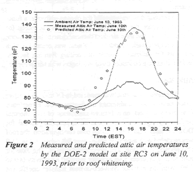
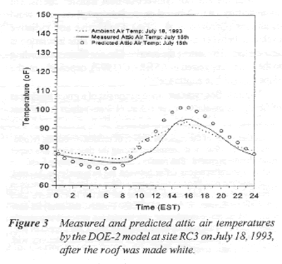
The attic air temperatures predicted by the DOE-2 model were compared with metered data in Figures 2 and 3. The graphs show the measured 15-minute ambient air and attic temperatures measured at Site 3 in West Florida in the summer of 1993 on two very hot days with similar solar radiation before and after the roof was whitened. Also plotted on the graphs are the predicted attic air temperatures from the model using the actual site weather data. The comparison shows that the simulation predicts the peak attic air temperatures reasonably well. The model still predicts a somewhat higher temperature than measured for the white roof case which should result in conservative estimates.
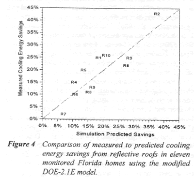
The success of the simulation on the impact of reflective roofing systems was determined by comparing the model’s prediction for cooling savings percentage for each of the eleven monitored Florida homes. This was accomplished by setting up individual building simulation decks which represented the each building’s thermal and operational characteristics. Two simulation runs were made, one with the initially measured roof reflectance and another with the reflective roof in place. Since the measurements were largely made between June and August, the predicted change in consumption was only tallied for this period. The individual savings predictions against those measured are shown in Figure 4. When taken overall, the DOE-2 model predicted an average 18.6% summer cooling energy savings for the 11 described cases in Central and South Florida against a measured savings of 19.3%. (40.1 kWh vs. 32.9 kWh/Day, 7.2 kWh/Day savings). Although short of the measured average reduction of 7.7 kWh/Day, the relative accuracy of the simulation gives confidence that the revised model will produce meaningful (although perhaps conservative) estimates for changes to roof solar reflectance. The model also tracks the major influence observed from the Florida field studies: percentage savings from reflective surfaces are higher with low ceiling insulation levels and flat roof geometries.
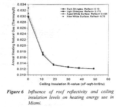
Figures 5 and 6 show how annual cooling and heating energy use is predicted to vary in Miami, Florida with differing levels of ceiling insulation (R-0 to R-49 hr ft2 oF/Btu or RSI 0 - 8.6) and roof reflectance (10 - 75%). For instance, in homes with no ceiling insulation (R-0) -- similar to many attic-less flat-roofed buildings built in South Florida in the 1950s -- the model predicts a 26% cooling savings from a reflective roof.
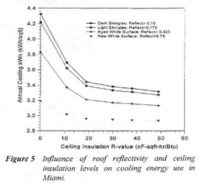
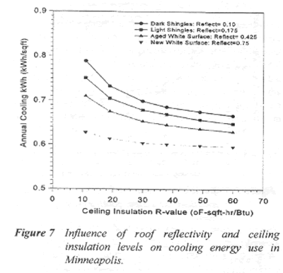
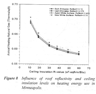
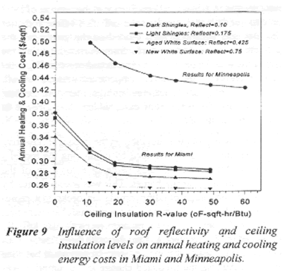
This influence of duct location is also seen. With R-19 (RSI 3.3) ceiling insulation and an attic duct system, the model predicts a 14% savings. On the other hand, with R-19 (RSI 3.3) insulation and the duct system located within the conditioned space, the model predicts only an 8% savings in Miami. A similar analysis for the other climatic extreme, Minneapolis, is shown in Figures 7 and 8. While cooling energy savings are still significant, their advantage is over matched by the increase of space heating in that location due to the detrimental impact of a reflective roof. Figure 9 shows the performance in terms of annual total space conditioning costs for both locations.
Climate Data and Prototypical Buildings
To address the variations of climate in the U.S., a total of 14 climate locations were simulated. The locations chosen were based on a cluster analysis of North American climates. This procedure considered heating and cooling degree days, solar radiation (T, the dimension- less ratio of annual extraterrestrial solar radiation to that received at the surface on a horizontal plane) and latent enthalpy hours (LEH, an indicator of humidity) for all typical meteorological year data for 125 standard metropolitan statistical areas in the U.S. (Anderson et al., 1984). The 14 chosen locations are Detroit, New York, Los Angeles, Atlanta, Houston, Ft. Worth, San Francisco, St. Louis, Minneapolis, Miami, Seattle, Fresno, Denver and Phoenix. The sites cover the gamut of meteorological variation within the United States including hot/cold, sunny/cloudy and humid/arid climate types.
Prototype buildings were created for the 14 climatic locations with simulations run for a base building and one with reflective roofing using TMY2 meteorological data (Marion and Urban, 1995). The physical description of the buildings were partly based on an analysis performed for the Gas Research Institute (Ritschard et al., 1992) which examined how foundation types, insulation levels and other characteristics varied by region. Other input was obtained from NAHB surveys, the ASHRAE 90.2 Standard and communication with state energy offices. It was deemed important to properly account for thermal integrity levels for the analysis, particularly with regard to ceiling insulation given the large interactions involved with changes to roof reflectance. To capture regional variation, three foundation types (slab, crawlspace and basement) were simulated with foundation models based on those developed by Huang et al. (1996B).
A single-story L-shaped floor plan with 1,500 square feet (139.4 m2) of conditioned floor space and an attached garage was used for the analysis. Although regional variations exist, it was decided to hold building geometry constant so that simulated differences could be attributed solely to differing levels of thermal efficiency, reflective roofing and duct system location. Analysis of two different sized prototypes revealed that the impact of reflective roofing scales well with changing roof and ceiling areas so this was not viewed as a problem. The fundamental simulation assumptions are detailed in Table 2.
Table 2 Building and Equipment Characteristics for Base-Case Buildings |
|
| Primary Characteristics | |
| Orientation | Long-axis faces north-south |
| Floor Area | 1,500 ft2 conditoned; foundation type varies with location |
| Roof | Asphalt shingles on plywood decking; 4/12 roof slope |
| Overhang | 2 feet around entire perimeter |
| Ceiling Insulation | Varies with location*; fiberglass over 1/2" sheet rock |
| Wall Construction | Frame construction: insulation level varies with location* |
| Solar Absorptance | 0.6, medium-tan color |
| Roof Absorptance | 0.9, dark gray asphalt shingles in base case |
| Windows | 224 ft2; 25% sash and frame with blinds/curtains, and some site shading; Window type varies with location*; U = 1.1 Btu/hr/ft2-°F, single, 0.5 double, 0.32 low-e |
| Infiltration | Sherman-Grimsrud algorithm; leakage based on climate and vintage
(Sherman et al., 1986) Specific Leakage Area (ft2 of leak per
ft2 floor area) Existing = 0.0005 < 4000 HDD; 0.0004 > 4000
HDD; New = 0.0004 < 4000 HDD; 0.0003> 4000 HDD |
| Heating and Cooling | |
| Heating | Natural gas furnace, 30,000 Btu/hr; Annual Fuel Utilization Efficiency (AFUE) = 75% (New), 70% (Existing) |
| Cooling | 3-ton AC, SEER= 8 Btu/W (Existing); SEER= 10 (New) |
| Distribution | Forced air system with duct location* dependant on foundation; 270 ft2 of supply ducts; 69 ft2 return; duct leakage 10% of fan flow (Existing), 5% (New); R-4 flex duct |
| Appliances | |
| Refrigerator | 1,500 kWh per year and part of internal gains |
| Lighting | Incandescent: 1,000 kWh/yr |
| Operation | |
| Heating Thermostat | 68 °F |
| Cooling Thermostat | 78 °F |
| Internal Heat Gains | 100 W per person/ Appliance gains average 648 W; Vary hourly on schedule |
| Natural Ventilation | Window ventilation @ 5 ACH when ambient temp >69° < 77° |
| *See Table 3 for specific values by location | |
We assumed three occupants in the home with typical electrical appliances and associated energy use. The specific end-use electrical demand profiles were taken from sub-metered appliance load data gathered from a large sample of homes in the Pacific Northwest (Pratt et al., 1989), but with only 90% of the loads assumed to take place within the conditioned space. The methodology is more fully described in Huang (1987).
Duct systems were assumed to be located in basements or crawlspaces if available and in attics in slab on grade homes. The site foundation type was selected by examining the 14 sites against typical regional foundation types as reported by Labs et al. (1988). Table 3 describes the location specific simulation assumptions:
Table 3 Site Prototype Characteristics |
||||||||||
Location |
Ceiling R-Value |
Wall R-Value |
Foundation Type |
Glazing Layers* |
Duct Location |
|||||
Exist. |
New |
Exist. |
New |
Exist. |
New |
Exist. |
New |
Exist. |
New |
|
| Detroit | 11 |
38 |
7 |
19 |
Basement |
2 |
2* |
Basement |
||
| New York | 11 |
38 |
7 |
19 |
Basement |
2 |
2* |
Basement |
||
| Los Angeles | 11 |
25 |
7 |
15 |
Slab |
1 |
2 |
Attic |
||
| Atlanta | 11 |
30 |
7 |
15 |
Crawl + |
Slab |
1 |
2 |
Crawl |
Attic |
| Houston | 11 |
30 |
0 |
11 |
Slab |
1 |
2 |
Attic |
||
| Ft. Worth | 11 |
30 |
0 |
11 |
Slab |
1 |
2 |
Attic |
||
| San Francisco | 11 |
30 |
7 |
15 |
Crawl |
Slab |
1 |
2 |
Attic |
|
| St. Louis | 11 |
30 |
7 |
15 |
Basement = |
2 |
2* |
Basement |
||
| Minneapolis | 22 |
44 |
11 |
22 |
Basement = |
2 |
2* |
Basement |
||
| Miami | 11 |
19 |
0 |
7 |
Slab |
1 |
1 |
Attic |
||
| Seattle | 19 |
38 |
7 |
19 |
Crawl + |
2 |
2* |
Crawl |
||
| Fresno | 11 |
30 |
7 |
15 |
Slab |
1 |
2 |
Attic |
||
| Denver | 11 |
38 |
7 |
19 |
Basement |
2 |
2* |
Basement |
||
| Phoenix | 11 |
30 |
7 |
15 |
Slab |
1 |
2 |
Attic |
||
| * Double-pane Low-e glass. + Crawl space floors are assumed to be uninsulated in existing homes; R-19 in new construction in Seattle. = Basement walls in Minneapolis are insulated to R-11 for new construction. |
||||||||||
Roof Solar Reflectance
The objective of the simulations was not to assess region wide potentials from changing surface reflectances, but rather to estimate the potential benefit of the choice of reflective roofing materials over conventional types and compare this option with adding additional attic insulation. The authors acknowledge that average roof solar reflectance varies with location. Observation suggests that lighter colors are already in evidence in warmer climates -- in part due to a inherent understanding of the influence of color on heat gain. However, with the advent of air conditioning, such practices may be on the decline.
Asphalt shingles now represent over half of all residential roofing installed in the United States (NRCA, 1993). The most popular colors are dark gray and earth-tones. Laboratory testing of 14 different colors of asphalt shingles showed solar reflectances were uniformly low varying from 5 - 25% with the former being black and the later a nominally white shingle (Parker et al., 1993). The reason for the low reflectances has much to do with the dark asphalt substrate on which the granules are impregnated. Even a specially prepared shingle, manufactured to be more white, had a tested reflectance of only 31%. Six of the more popular gray and brown colors had a tested average solar reflectance of only 10%. This suggests that a solar absorptance of 0.90 could be used to model current practice.
Obviously, a simple no-cost option would be to choose light-colored shingles (25% solar reflectance). Other time-proven options to improve residential roof solar reflectance are to choose white concrete tiles or white standing-seam metal for new or re-roofs. Tested samples show that it is possible to achieve a 75% initial solar reflectance with such materials (Parker et al., 1993B).
One large issue associated with potential benefits from reflective surfaces is that surface reflectances may degrade over time due to aging and weathering. Several studies indicate that white surfaces can lose as much as 20% of their reflectance in two years, although further degradation slows after that point (Bretz and Akbari, 1993; Byerley and Christian, 1994; Parker et al., 1995). Anecdotal observation suggests that degradation is strongly affected by surface smoothness, pitch, local humidity and microbial resistance. Smooth metal roofs seem to have the least problems in this regard. The authors are familiar with several homes in Florida with white standing-seam metal roofs which appear pristine after five years exposure.
However, given the uncertainty in long-term performance, and the contentious debate surrounding this issue, we used a simple conservative assumption. We assumed that the aged performance of reflective surfaces on residences would be mid-way between the initial reflectance (75% for white tile or metal and 25% for white shingles) and the reference base (10%). The foregoing assumptions were used to set up the cases to be analyzed to determine relative impact of white roof surfaces. As a point of reference, we also analyzed adding another three inches (R-11 or 7.6 cm) of ceiling insulation to new and existing buildings to examine performance relative to a change in roof solar reflectance.
Table 4 Cases for Analysis |
||
Configuration |
Description |
Solar Reflectance |
| Base | Gray/brown asphalt shingle | 0.100 |
| Base w/ Insulation | Base + added R-11 ceiling insulation | 0.100 |
| White Shingle | White asphalt shingle | 0.175* |
| White Roof | New white tile/metal | 0.750 |
| White Roof | Weathered white tile/metal | 0.425* |
*Weathered value. |
||
The costs for electricity and natural gas are taken from national residential averages for 1996 (EIA, 1997): $0.084/kWh and $0.63/therm. It was desirable to use average rather than local energy prices so that results from specific locations be based on climatic or building related differences. Although no life- cycle cost analysis was undertaken, the incremental cost of white standing-seam metal over a Class-A asphalt shingle roof is approximately $1.00 per square foot ($11/m2); the incremental cost for concrete barrel tile installed is about $2.00 (Means, 1997). White asphalt shingles have no incremental cost over other colors. As a point of reference, the same residential cost estimator shows an average incremental cost for R-11 (RSI 1.9) batt insulation (eg. from R-19 to R30 insulation) of approximately $0.25/square foot ($2.70/m2) including overhead and profit.
Results
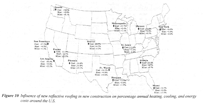
Results of the simulation analysis of reflective roofing are presented in Table 5 for new and existing construction in each of the locations. The table gives the annual heating (therms of natural gas) and cooling energy use (kWh) normalized by floor area as well as total yearly energy costs based on national average energy prices. Figure 10 provides a graphical representation of the impact of reflective roof systems in new construction on an annual heating and cooling energy and costs around the U.S.
Table 5 Simulation Results for Reflective Roof Analysis |
|||||||||||
Location |
Base |
White Shingle |
New White Roof |
Weathered White Roof |
Base + R-11 |
||||||
|
Reflect. = 0.10 |
Reflect. = 0.175 |
Reflect. = 0.75 |
Reflect. = 0.425 |
Reflect. = 0.10 |
|||||||
Exist. |
New |
Exist. |
New |
Exist. |
New |
Exist. |
New |
Exist. |
New |
||
Detroit |
kWh/ft2 therms/ft2 cost/ft2 |
0.801 0.700 $0.508 |
0.500 0.415 $0.303 |
0.773 0.702 $0.507 |
0.492 0.417 $0.304 |
0.590 0.722 $0.504 |
0.417 0.427 $0.304 |
0.696 0.711 $0.506 |
0.463 0.421 $0.304 |
0.717 0.649 $0.469 |
0.490 0.407 $0.298 |
New York |
kWh/ft2 therms/ft2 cost/ft2 |
1.172 0.524 $0.429 |
0.656 0.310 $0.250 |
1.145 0.526 $0.428 |
0.645 0.311 $0.250 |
0.917 0.546 $0.421 |
0.551 0.322 $0.249 |
1.049 0.534 $0.425 |
0.607 0.316 $0.250 |
1.076 0.481 $0.393 |
0.643 0.303 $0.245 |
Los Angeles* |
kWh/ft2 therms/ft2 cost/ft2 |
0.333 0.112 $0.099 |
0.198 0.052 $0.049 |
0.309 0.113 $0.097 |
0.189 0.053 $0.049 |
0.141 0.118 $0.086 |
0.120 0.054 $0.043 |
0.233 0.114 $0.091 |
0.146 0.053 $0.046 |
0.260 0.098 $0.084 |
0.181 0.049 $0.046 |
Atlanta+ |
kWh/ft2 therms/ft2 cost/ft2 |
2.122 0.366 $0.409 |
1.508 0.176 $0.238 |
2.080 0.367 $0.406 |
1.471 0.176 $0.234 |
1.701 0.382 $0.384 |
1.176 0.184 $0.215 |
1.926 0.373 $0.397 |
1.349 0.179 $0.226 |
1.954 0.340 $0.378 |
1.470 0.170 $0.231 |
Houston+ |
kWh/ft2 therms/ft2 cost/ft2 |
4.014 0.259 $0.500 |
2.479 0.083 $0.261 |
3.940 0.260 $0.495 |
2.438 0.083 $0.257 |
3.327 0.269 $0.449 |
2.095 0.086 $0.230 |
3.688 0.264 $0.476 |
2.297 0.085 $0.246 |
3.830 0.249 $0.479 |
2.439 0.080 $0.255 |
Ft. Worth+ |
kWh/ft2 therms/ft2 cost/ft2 |
3.967 0.379 $0.571 |
2.431 0.125 $0.283 |
3.903 0.381 $0.568 |
2.387 0.125 $0.279 |
3.312 0.395 $0.527 |
2.039 0.130 $0.253 |
3.660 0.386 $0.550 |
2.239 0.127 $0.268 |
3.815 0.363 $0.549 |
2.385 0.120 $0.276 |
| San Francisco | kWh/ft2 therms/ft2 cost/ft2 |
0.181 0.287 $0.196 |
0.127 0.126 $0.090 |
0.173 0.288 $0.196 |
0.123 0.126 $0.090 |
0.125 0.305 $0.203 |
0.105 0.131 $0.091 |
0.152 0.294 $0.198 |
0.115 0.128 $0.090 |
0.163 0.262 $0.179 |
0.123 0.121 $0.087 |
| St. Louis | kWh/ft2 therms/ft2 cost/ft2 |
1.813 0.518 $0.479 |
1.169 0.314 $0.296 |
1.776 0.520 $0.477 |
1.153 0.315 $0.295 |
1.461 0.538 $0.462 |
1.104 0.324 $0.289 |
1.645 0.527 $0.470 |
1.091 0.319 $0.293 |
1.671 0.477 $0.441 |
1.141 0.305 $0.288 |
| Minneapolis | kWh/ft2 therms/ft2 cost/ft2 |
0.743 0.713 $0.512 |
0.620 0.463 $0.344 |
0.726 0.715 $0.511 |
0.611 0.464 $0.344 |
0.593 0.733 $0.512 |
0.535 0.474 $0.344 |
0.673 0.722 $0.511 |
0.579 0.468 $0.344 |
0.712 0.685 $0.491 |
0.611 0.455 $0.338 |
| Miami + | kWh/ft2 therms/ft2 cost/ft2 |
5.013 0.030 $0.440 |
3.444 0.013 $0.297 |
4.935 0.030 $0.433 |
3.392 0.013 $0.293 |
4.291 0.031 $0.380 |
2.960 0.014 $0.257 |
4.673 0.030 $0.411 |
3.211 0.014 $0.279 |
4.854 0.028 $0.425 |
3.372 0.012 $0.291 |
| Seattle | kWh/ft2 therms/ft2 cost/ft2 |
0.385 0.426 $0.301 |
0.305 0.229 $0.170 |
0.375 0.428 $0.301 |
0.301 0.230 $0.170 |
0.297 0.440 $0.302 |
0.255 0.238 $0.171 |
0.343 0.433 $0.302 |
0.281 0.233 $0.170 |
0.364 0.407 $0.287 |
0.299 0.223 $0.166 |
| Fresno + | kWh/ft2 therms/ft2 cost/ft2 |
3.161 0.269 $0.435 |
2.045 0.136 $0.257 |
3.073 0.270 $0.428 |
1.997 0.137 $0.254 |
2.329 0.285 $0.375 |
1.607 0.143 $0.225 |
2.766 0.276 $0.406 |
1.839 0.139 $0.242 |
2.896 0.245 $0.397 |
1.991 0.131 $0.250 |
| Denver | kWh/ft2 therms/ft2 cost/ft2 |
1.091 0.543 $0.434 |
0.640 0.312 $0.250 |
1.053 0.545 $0.432 |
0.627 0.313 $0.250 |
0.753 0.572 $0.424 |
0.501 0.326 $0.247 |
0.927 0.559 $0.430 |
0.574 0.318 $0.249 |
0.959 0.498 $0.394 |
0.623 0.305 $0.240 |
| Phoenix + | kWh/ft2 therms/ft2 cost/ft2 |
5.967 0.116 $0.574 |
3.880 0.052 $0.359 |
5.858 0.117 $0.566 |
3.821 0.052 $0.354 |
4.901 0.122 $0.489 |
3.313 0.054 $0.312 |
5.471 0.118 $0.534 |
3.614 0.053 $0.337 |
5.596 0.102 $0.534 |
3.804 0.049 $0.351 |
| * Annual energy cost/ft2 is less for
new construction with a new reflective roof than adding an additional
increment of R-11 insulation. + As above, but also lower cost for a weathered roof in new construction rather than adding R-11 |
|||||||||||
Discussion
Review of the results above reveals the following influences:
-
In all locations, reflective roofs reduce space cooling requirements. The percentage annual cooling savings varied from 13% (new construction in St. Louis) to 58% (existing construction in Los Angeles). The percentage by which heating requirements were increased in existing housing by reflective roofing varied from 3% in Miami to 6% in San Francisco.
-
Except in the northernmost locations (Minneapolis and Detroit), and cool and cloudy locations (Seattle and San Francisco), the combined cost of heating and cooling was shown to be lower for reflective roof surfaces than conventional ones.
-
The advantage of light colored roof surfaces is greatest in the lower latitudes. In locations where the annual energy cost savings was higher for new construction for a new reflective roof than adding another increment of insulation, an asterisk (*) is shown in the table. This was true of Los Angeles, Atlanta, Houston, Ft. Worth, Miami, Fresno and Phoenix. Two asterisks (**) indicate that a weathered white roof produces greater savings as well. These locations are all below 37 degrees north latitude.
-
Cooling energy savings were greatest in existing housing which tends to have lower ceiling insulation levels.
-
The comparative performance of white roofs over adding further insulation, is more favorable in new construction where higher levels of ceiling insulation typically will be present.
-
Percentage savings in space cooling from white roofs was greatest in moderate sunny climates. A new white roof on an existing home in Los Angeles was predicted to reduce air conditioning energy by 58% while increasing space heating consumption by only 5%.
-
The absolute cooling savings of reflective roofs was greatest in the hottest and sunniest locations. Annual cooling energy savings in Phoenix were for existing housing 1.07 kWh/ft2 (11.4 kWh/m2).
-
In the hottest locations (Phoenix and Miami) choice of white rather than gray shingles for new construction provides more than 60% of the annual energy savings produced by adding R-11.
Conclusions
A detailed model was developed using the DOE-2.1E building energy simulation to estimate the benefits from solar reflective roofing systems in residential housing in North America. Special modifications were made, enabling the DOE-2 program to simulate the key thermal processes that have been poorly modeled to date. This includes a detailed model of a residential attic, potential interaction with the thermal distribution system when located in this space and assessment of the temperature dependence of insulation conductivity with mean temperature. The model was shown to provide reasonable agreement to measured data taken from Florida test homes.
The model was then used to simulate the impact of reflective roofing in 14 different climates around the United States. A residential prototype building was modified in terms of its foundation, duct system location and thermal integrity to reflect both new and existing housing across climatic regions. Results indicated that large cooling energy benefits from reflective roofing in sites in the “sun belt” below 37 degrees north latitude. In southern climates the annual space conditioning energy savings for a new house with weathered reflective roofing system were often found to outweigh the reduction predicted from an added three inches (R-11 hr ft2 oF/Btu or RSI - 1.9) of insulation.
The savings of white roofs are influenced by duct system location. The predicted annual cooling energy savings for a white roof for a new home in Miami with R-19 ceiling insulation was 14% (730 kWh) with an attic duct system. However, it was only 8% (362 kWh) with the duct system located in the conditioned space.
In all locations, reflective roofing (even when weathered) was found to be very effective at reducing cooling loads. The largest percentage savings was in existing housing in Los Angeles -- a 58% reduction in annual cooling energy. The largest absolute savings of 1.07 kWh/ft2 (11.4 kWh/m2) was in Phoenix, the hottest and sunniest location. The relative advantage of reflective roofing systems against added insulation was found to be largely a function of the relative magnitude of cooling against heating. In climates where heating needs dominate, above 40 degrees north latitude, there was little advantage to be gained from reflective roofing and in the coldest locations, added insulation was clearly a better choice. Similarly, in the southernmost locations analyzed, such as Phoenix and Miami, reflective roofing systems even when strongly weathered, produced greater savings than adding R-11 (RSI - 1.9) to typical ceiling insulation levels. Our results underscore the need for climate-related provision for reflective roof surfaces as an energy efficiency tradeoff within the ASHRAE Standard 90.2 energy code for residential buildings.
Acknowledgment
This research has been co-funded by the Florida Energy Office in support of the Building Design Assistance Center and the Office of Building Technologies of the U.S. Department of Energy. Their joint sponsorship is gratefully acknowledged. Hashem Akbari (LBNL) provided many useful comments during the analysis and Wanda Dutton skillfully prepared the manuscript and report graphics. Finally, special thanks to the many individuals in institutions around the country who helped create realistic regional prototypes for the analysis.
References
Akbari, H., Taha, H. and Sailor, D., 1992. "Measured Savings in Air Conditioning from Shade Trees and White Surfaces," Proceedings of the 1992 ACEEE Summer Study on Energy Efficiency in Buildings, American Council for an Energy Efficient Economy, Washington D.C., Vol. 9, p. 1.
Akbari, H., Rosenfeld, A.H. and Taha, H., 1990. "Summer Heat Islands, Urban Trees and White Surfaces," ASHRAE Transactions, Vol. 96, Pt. 1, American Society of Heating, Refrigeration and Air Conditioning Engineers, Atlanta, GA.
Anderson, R.W., 1989. "Radiation Control Coatings: An Under-utilized Energy Conservation Technology for Buildings," ASHRAE Transactions Vol. 95, Pt. 2, 1989.
ASHRAE, 1993. Handbook of Fundamentals, American Society of Heating, Refrigeration and Air Conditioning Engineers, Chapter 22, Table 1, Atlanta, GA.
Bansal, N.K., Garg, S.N. and Kothari, S., 1992. "Effect of Exterior Surface Color on the Thermal Performance of Buildings," Building and Environment, Permagon Press, Vol. 27, No. 1, p. 31-37, Great Britain.
Bretz, S. and Akbari, H., 1993. Durability of High Albedo Coatings, LBL-34974, Lawrence Berkeley Laboratory, Berkeley, CA.
Byerley, A.R. and Christian, J.E., 1994. "The Long-Term Performance of Radiation Control Coatings," Proceedings on the 1994 Summer Study on Energy Efficiency in Building, Vol. 5, p. 59, American Council for an Energy Efficient Economy, Washington, DC.
EIA, 1997. Monthly Energy Review, March, 1997, DOE/EIA-0035(97/03), Energy Information Administration, Washington D.C.
Gartland, L.M., Konopacki, S.J. and Akbari, H., 1996. “Modeling the Effects of Reflective Roofing,” Proceedings of the 1996 ACEEE Summer Study on Energy Efficiency in Buildings, Vol. 4, p. 117, American Council for an Energy Efficient Economy, Washington D.C.
Givoni, B. and Hoffman, M.E., 1968. "Effect of Building Materials on Internal Temperatures," Research Report, Building Research Station, Technion Haifa.
Givoni, B., 1976. Man, Climate and Architecture, Applied Science Publishers Ltd., London.
Griggs, E.I, and Shipp, P.H., 1988. "The Impact of Surface Reflectance on the Thermal Performance of Roofs: An Experimental Study," ASHRAE Transactions, Vol. 94, Pt. 2, Atlanta,GA.
Gu, L., Cummings, J.E., Swami, M.V., Fairey, P.W. and Awwad, S., 1996. Comparison of Duct System Computer Models That Could Provide Input to the Thermal Distribution System Standard Method of Test (SPC-152P), FSEC-CR-929-96, ASHRAE Project 852-RP, Florida Solar Energy Center, Cocoa, FL.
Hageman, R. and Modera, M.P., 1996. “Energy Savings and HVAC Capacity Implications of a Low-Emissivity Interior Surface for Roof Sheathing,” Proceedings of the 1996 ACEEE Summer Study on Energy Efficiency in Buildings, Vol. 1, p. 117, American Council for an Energy Efficient Economy, Washington D.C.
Huang, J. and Vincent, B., 1996. Analysis of the Energy Performance of Cooling Retrofits in Sacramento Housing Redevelopment Agency using Monitored Data and Computer Simulations, J Huang and Associates, prepared for California Energy Commission, April 1, 1996.
Huang, J., Bazjanac, V. and Feustel, H., 1996. Evaluation of Simplified Methods for Calculating Foundation Heat Flows in Annual Building Energy Simulations, J Huang and Associates, prepared for California Energy Commission, August 15, 1996.
Huang, J., 1987. Methodology and Assumptions for Evaluating Heating and Cooling Energy Requirements in New Residential Single Family Buildings, LBL-19128, Lawrence Berkeley National Laboratory, Berkeley, CA.
Jump, D.A., Walker, I.S. and Modera, M.P., 1996. “Measurements of Efficiency and Duct Retrofit Effectiveness in Residential Forced Air Distribution Systems,” Proceedings of the ACEEE 1996 Summer Study on Energy Efficiency in Buildings, Vol. 1, p. 147, American Council for an Energy Efficient Economy, Washington D.C.
Konopacki, S., Akbari, H., Gabersok, S., Pomorantz, M., Gartland, L.,
and Moezzi, M., 1996. Energy and Cost Benefits from Light Colored Roofs
in 11 U.S. Cities, Lawrence Berkeley Laboratory, LBL-39433, Berkeley,
CA.
Labs, K., Carmody, J., Sterling, R., Shen, L., Huang, J. and Parker,
D., 1988. Building Foundation Handbook, ORNL/Sub/86-72143/1, Oak Ridge
National Laboratory, Oak Ridge, TN.
Langewiesche, W., 1950 “Your House in Florida,” House Beautiful, January, 1950, p.74.
Lapujade, P.G., 1994. On Site Roof Reflectance Measurement Methodology: Theory and Limitations, FSEC-RR-28-94, Florida Solar Energy Center, Cocoa, FL.
Lauvray, T.L., 1978. “Experimental Heat Transmission Coefficients for Operating Air Duct Systems,” ASHRAE Journal, June, 1978, Atlanta, GA.
Marion, W. and Urban, K., 1995. User’s Manual for TMY2: Typical Meteorological Years, National Renewable Energy Laboratory, Golden, CO.
Levinson, R., Akbari, H. and Gartland, L.M., 1996. “Impact of the Temperature Dependency of Fiberglass Insulation R-Value on Cooling Energy Use in Buildings,” Proceedings of the ACEEE 1996 Summer Study on Energy Efficiency in Buildings, Vol. 10, p. 85, American Council for an Energy Efficient Economy, Washington D.C.
Means, R.S., 1997. Means Residential Cost Data, 16th Annual Edition, Kingston, MA.
Parker, D.S.,Barkaszi, Jr., S.F., Chandra, S. and Beal, D., 1995. “Measured Energy Savings from Reflective Roofing Systems in Florida: Field and Laboratory Research Results, Thermal Performance of the Exterior Envelopes of Buildings VI, U.S. DOE/ORNL/BETEC, December 4-8, 1995, Clearwater, FL.
Parker, D.S., Fairey, P.W. and Gu, L., 1993. “Simulation of the Effects of Duct Leakage and Heat Transfer on Residential Space Cooling Energy Use,” Energy and Buildings, 20, p. 97-113, Elsevier Sequoia, Netherlands.
Parker, D.S., McIlvaine, J.E.R., Barkaszi, S.F. and Beal, D.J., 1993A. Laboratory Testing of the Reflectance Properties of Roofing Materials, FSEC-CR-670-93, Florida Solar Energy Center, Cape Canaveral, FL.
Parker, D.S., Cummings, J.B., Sherwin, J.S., Stedman, T.C. and McIlvaine, J.E.R., 1993B. Measured Air Conditioning Electricity Savings from Reflective Roof Coatings Applied to Florida Residences, FSEC-CR-596-93, Florida Solar Energy Center, Cape Canaveral, FL.
Parker, D.S., Fairey, P.F. and Gu, L., 1991. “A Stratified Air Model for Simulation of Attic Thermal Performance,” Insulation Materials: Testing and Applications, ASTM STP-1116, p. 44, American Society of Testing and Materials, Philadephia, PA.
Reagan, J.A. and Acklam, D.M., 1979. "Solar Reflectivity of Common Building Materials and its Influences on the Roof Heat Gain of Typical Southwestern U.S. Residences," Energy and Buildings No. 2, Elsevier Sequoia, Netherlands.
Ritschard, R.L., Hanford, J.W. and Sezgen, A.O., 1992. Single Family Heating and Cooling Requirements: Assumptions, Methods and Summary Results, GRI-91/0236, prepared by LBNL for Gas Research Institute, March, 1992.
Sherman, M.H., Wilson, D.J. and Kiel, D.E., 1986. “Variability in Residential Air Leakage,” Measured Air Leakage in Buildings ASTM STP-904, American Socieity of Testing and Materials, Philadelphia, PA.
Taha, H., Akbari, H., Rosenfeld, A.H. and Huang, J., 1988. "Residential Cooling Loads and the Urban Heat Island--the Effects of Albedo," Building and Environment, Vol 23, No. 4, Permagon Press, Great Britain.
Taha, H. Sailor, D. and Akbari, H., 1992. High Albedo Materials for Reducing Building Cooling Energy Use, Lawrence Berkeley Laboratory Report No. LBL-31721, Lawrence Berkeley Laboratory, Berkeley, CA.
Turner, W.C. and Malloy, J.F., 1981. Thermal Insulation Handbook, McGraw-Hill Book Company, NY.
Walker, I.S., Forest, T.W. and Wilson, D.J., 1995. “ A Simple Calculation Method for Attic Ventilation Rates,” Proceedings of the 16th AIVC Conference, Vol. 1, p. 221-231, Air Infiltration and Ventilation Centre, Palm Springs, CA.
Wilkes, K.E., 1981. “Thermophysical Properties Data Base Activities at Owens-Corning Fiberglas,” Proceedings of the ASHRAE/DOE/ORNL Conference, ASHRAE SP28, p. 622-677, Oak Ridge National Laboratories, Oak Ridge, TN.
© 2007-2014 University of Central Florida. The Florida Solar Energy Center (FSEC)
is a research institute of the
University of Central Florida.
For more information about FSEC, please contact us or learn more about us.
Find us on Facebook!